5G(NR): Frame structure( Slots and symbols Formats)
5G NR CORESET
UE 5G NR Search Space
5G_NR_SLIV:
PDSCH Resource Allocation in Time-Domain
5G-NR: MIB
5G NR: DCI Formats
5G-NR: Carrier Aggregation (CA)
5G-NR: Channels
5G-NR: SIGNALLING RADIO BEARERS
5G NR Bandwidth Part (BWP)
5G(NR)-GUTI, SUPI, SUCI
MSG1 – PRACH in 5G NR:
What is ARQ and HARQ?
5G (NR): DAPS Handover
Image Merger Tool
Drag & Drop Images Here
The Pro Version of the Image Merger tool brings a new level of power, speed, and creative control for users who want more than just simple image merging. This upgraded tool is built for bloggers, graphic creators, students, photographers, and professionals who want fast, high‑quality results directly inside their browser and WordPress website.
Below are the highlighted features of the Pro Edition:
✨ 1. New Modern UI (User Interface)
The Pro version introduces a sleek, minimal, and fully responsive interface inspired by premium photo editing apps.
Key benefits:
Clean and distraction-free workspace
Mobile-friendly and touch-optimized
Smooth animations and panel transitions
Drag‑and‑drop visual grid for easy image arrangement
This polished interface makes the tool feel like a professional desktop application running inside your blog.
✨ 2. Background Remover AI (Advanced On‑Device Processing)
Remove backgrounds instantly using AI-powered segmentation — right in your browser.
What makes it special:
Works offline (no server upload)
Preserves privacy and speed
Detects subjects accurately
Produces clean transparent PNGs
This feature is ideal for ecommerce photos, thumbnails, portraits, and product cutouts.
✨ 3. Add Logo Watermark (Brand‑Ready Output)
Protect your content or promote your brand by adding your custom logo watermark with full control.
Supported options:
Upload PNG/SVG logos
Adjust opacity
Move logo to any corner
Resize using slider controls
This makes it perfect for bloggers, influencers, and small businesses who want branded visuals.
✨ 4. Auto‑Resize Images (Smart Scaling Engine)
The tool can automatically resize and optimize all imported images to maintain a consistent layout.
Features include:
Maintain aspect ratio
Fit-to-grid scaling
Auto‑sharpening
Smart width/height uniform resizing
This ensures all images align perfectly in grids, collages, or long vertical documents.
✨ 5. Cloud Upload Support (Pro-Cloud Ready)
With cloud support, users can import images not just from their device but also from cloud platforms (where supported):
Compatible options (based on browser support):
Google Drive
OneDrive
Dropbox
iCloud (on Apple devices)
This is especially useful for users working across multiple devices or storing assets online.
✨ 6. Export Options: JPG, PNG, and PDF
The Pro version supports multiple export formats for different use cases:
✔ PNG — Best for transparent or high-quality images ✔ JPG — Best for blogs, lightweight sharing, and SEO ✔ PDF — Perfect for printables, documents, and portfolios
The export engine is optimized for high resolution, sharpness, and file size balance.
✨ 7. Pro Version WordPress Plugin (Complete Integration)
The Pro version comes as a fully functional WordPress plugin with:
Shortcode support
Gutenberg block support
Auto UI loader
Dedicated settings panel
Secure script handling
100% browser-based processing
Your users get a seamless experience inside any WordPress page — no external apps required.
Non‑Terrestrial Networks (NTN) are one of the biggest breakthroughs introduced in 3GPP Release‑17, making 5G capable of connecting users beyond Earth-based towers. Unlike traditional networks that depend on land-based cell sites, NTNs bring connectivity from space and high-altitude platforms, enabling coverage in oceans, mountains, deserts, rural areas, and disaster zones.
3GPP officially defines NTN as communication networks that rely on LEO, MEO, GEO satellites, HAPS platforms, and UAV-based relays to deliver 5G service from above the Earth’s surface.
Why NTN Matters in Modern 5G?
Traditional terrestrial networks cannot reach everywhere. Factors like geography, low population density, and infrastructure cost create coverage gaps. NTNs bridge these gaps using satellites and high-altitude systems, improving:
Global broadband access
Emergency & disaster communication
Maritime & aviation services
IoT expansion
Positioning & timing support
3GPP studies highlight that maintaining uplink synchronization, updating satellite ephemeris, and adapting SI (System Information) delivery — especially SIB19 — are essential to maintain stable NTN connectivity.
Types of NTN Platforms
NTN platforms listed by 3GPP include:
1. Low Earth Orbit (LEO) satellites
500–2000 km altitude
Lower latency
Requires large constellations
2. Medium Earth Orbit (MEO) satellites
8000–20,000 km
Balanced latency and coverage
3. Geostationary Orbit (GEO) satellites
35,786 km
Huge coverage, but higher latency
4. High-Altitude Platforms (HAPS)
Such as balloons or solar-powered aircraft hovering around 20 km altitude.
5. UAV-based Aerial Relays
Used in emergency coverage.
NTN research shows rapid advancements in SIB19 optimization, including compressed ephemeris, AI-assisted beam prediction, and on-board GNSS receivers to reduce error and enhance UE tracking.
SIB19 – The Heart of NTN System Information
SIB19 is a unique NTN-specific System Information Block introduced in 5G Release‑17. It includes:
Satellite orbit parameters
Timing correction data
GNSS assistance
Beam IDs / satellite identifiers
UL‑Sync validity timers
3GPP research confirms SIB19 is essential to maintain uplink synchronization in NTN because satellite movement constantly alters delay and Doppler shifts. As a result, UE must periodically reacquire SIB19 based on defined SI periodicity and network algorithms.
How NTN SI (System Information) Works ?
SIB19 is transmitted using SI‑RNTI, same as legacy SIBs(SIB1, SIB2,SIB3, SIB4…). All NTN UEs decode SIB19 using downlink PDSCH just like normal SIBs. However, NTN SI scheduling faces challenges:
Satellite movement → dynamic SI timing
Large RTT (Round Trip Time) → scheduling offsets
SI-window alignment with other SIBs (SIB2–SIB5)
3GPP ensures SIB19 avoids SI-window overlap by defining specific window position rules and scheduling behavior.
Key Challenges in NTN
Propagation Delay Satellite links create much higher RTT.
Doppler Shift LEO satellites move at ~7.5 km/s → high frequency shifts.
Beam Movement Rapidly changing beam footprints require tracking.
Power Constraints Handsets must decode weak signals from hundreds of kilometers away.
System Information Complexity SIB19 must carry more dynamic information than terrestrial SIBs.
Per 5G NR spec, RA‑RNTI is derived from PRACH occasion indices: t_id (time), f_id (frequency), and uplink carrier index. Formula: 1 + t_id + 14×f_id + 14×80×ul_carrier_id.
RA‑RNTI (Random Access RNTI) — Short Description
RA‑RNTI is a temporary identifier used in 5G NR during the Random Access Procedure. It uniquely represents a UE’s PRACH transmission occasion (defined by time index t_id and frequency index f_id), allowing the gNB to identify which UE sent the RA preamble.
Once calculated using the PRACH occasion, the gNB uses this RA‑RNTI to send the Random Access Response (RAR) to the correct UE.
Tip: This tool parses the DCI bit payload using dynamic field sizes derived from 3GPP formulas (RBG sizes, RIV, etc.). It does not perform CRC/Polar decoding.
MCS tables and Qm/R come from TS 38.214 §5.1.3.1 Tables 5.1.3.1‑1/‑2/‑3. [2](https://www.sharetechnote.com/html/5G/5G_MCS_TBS_CodeRate.html)
N’RE and 156‑RE cap per PRB follow the examples used in TS 38.214 sources (RE accounting within a PRB). [3](https://www.sqimway.com/nr_pdsch.php)
TBS uses the §5.1.3.2 two‑branch method with small‑block threshold 3824 bits. The default “Round‑to‑6‑bit” option mirrors common reference tools; request “spec‑table” if you need the exact discrete set. [4](https://www.rfwireless-world.com/calculators/5g-nr-tbs-calculation)[5](https://5g-tools.com/5g-nr-tbs-transport-block-size-calculator/)
Background (you can paste near the widget)
Qm/R selection: Choose the MCS table and index; Qm and target code rate R come from TS 38.214 §5.1.3.1 (Tables 1–3).
RE accounting: For an allocation of Nsymb,sh symbols, the usable RE/PRB is N’RE = 12·Nsymb,sh − NDMRS − Noh, capped to 156 RE/PRB.
TBS determination: Form Ninfo = NRE × R × Qm × ν × tbScaling, then apply the ≤ 3824 / > 3824 procedures in TS 38.214 §5.1.3.2. (This calculator uses the common 6‑bit quantization for small TBS; on request, I can switch to a spec‑exact discrete set.)
PCI range is 0–1007 (1008 identities), structured as 336 groups × 3 identities per group (NID(1), NID(2)). [1](https://www.etsi.org/deliver/etsi_ts/138200_138299/138211/18.07.00_60/ts_138211v180700p.pdf)[2](https://www.rfwireless-world.com/calculators/5g-nr-physical-layer-cell-id-calculator)
Mapping: PCI = 3×NID(1) + NID(2), with NID(1)∈[0,335] from SSS and NID(2)∈{0,1,2} from PSS. [1](https://www.etsi.org/deliver/etsi_ts/138200_138299/138211/18.07.00_60/ts_138211v180700p.pdf)[3](https://www.telecomtrainer.com/5g-nr-physical-cell-id-pci-explained-pss-sss-and-synchronization/)
Cell search derives PSS/SSS (hence PCI) inside the SSB burst as per 38.211 procedures. [1](https://www.etsi.org/deliver/etsi_ts/138200_138299/138211/18.07.00_60/ts_138211v180700p.pdf)
Note:
1- What is PCI? A physical‑layer cell identity used by UE during cell search and synchronization; it’s derived from PSS/SSS in the SSB burst.
2- Ranges and formula:NID(1)N_{\text{ID}}^{(1)}NID(1) from SSS ∈ [0,335], NID(2)N_{\text{ID}}^{(2)}NID(2) from PSS ∈ {0,1,2}, and PCI ∈ [0,1007], with PCI=3NID(1)+NID(2)\text{PCI} = 3N_{\text{ID}}^{(1)} + N_{\text{ID}}^{(2)}PCI=3NID(1)+NID(2).
Thermal noise uses kTB (−174 dBm/Hz @ 290 K) with temperature scaling. [2](https://www.wirelessbrew.com/tools/thermal-noise/)[3](https://www.onesdr.com/calculate-ktb-noise-power/)
Receiver sensitivity = noise floor + required SNR. Reference sensitivity is a 3GPP KPI (TS 38.101‑1); exact targets depend on test channel/MCS, hence SNRreq is user input. [4](https://www.etsi.org/deliver/etsi_ts/138100_138199/13810101/17.18.00_60/ts_13810101v171800p.pdf)
Fixed Conditions
Tx/Rx & Losses
Target
Max FSPL allowed: dB
Max Range (km): km
What is 5G NR Link‑Budget?
A Link‑Budget in 5G NR is a complete, end‑to‑end accounting of all gains and losses a radio signal experiences as it travels from the transmitter (gNB/UE) to the receiver (UE/gNB).
It answers two core engineering questions:
Will the received signal be strong enough to meet the required SNR for decoding?
What is the maximum coverage distance for a given transmit power, frequency, bandwidth, and environment?
Link‑budget is essential for:
Cell planning & coverage prediction
Network optimization
gNB/UE sensitivity assessment
Propagation model comparison
Determining downlink vs uplink imbalance
Why Link‑Budget Matters in 5G NR
5G uses higher frequencies (FR1 up to 7.125 GHz, FR2 up to 52.6 GHz), massive MIMO antennas, beamforming, and wide bandwidths — all of which impact signal strength.
Higher frequencies → higher free‑space path loss Wider bandwidth → higher thermal noise Beamforming → higher antenna gain NR numerology & MIMO → different SNR and performance targets
This makes link‑budget more important in NR compared to LTE.
A number system is a way to represent numbers using a specific set of digits. In computers and digital electronics, different number systems are used to store and process data.
Understanding SINR in 5G Networks: The Key to Ultra-Reliable Performance
Signal-to-Interference-plus-Noise Ratio, or SINR, measures how well a 5G signal stands out against disruptions. In 5G networks, this ratio decides if you get the fast speeds and low delays that make the tech shine. Past generations like 4G focused on basic coverage, but 5G demands top-notch SINR to handle heavy data loads from videos, smart devices, and real-time apps. Without strong SINR, those promises of gigabit speeds fade fast. Think of it as the heartbeat of your connection—weak SINR means spotty service, while high levels unlock the full power of 5G.
Defining SINR: The Essential Measurement for Wireless Health
SINR tells you the quality of your wireless link in simple terms. It uses this formula: SINR equals signal power divided by the sum of interference and noise. In 5G, a high value means clean data flow; low ones lead to errors and slow downs.
The signal power, or S, is the strength of the main transmission reaching your device. It comes from the base station’s pilot signals, measured as RSRP in 5G terms. Strong S boosts your download speeds and video calls stay smooth.
S: The Desired Signal Power
RSRP gauges the raw power of reference signals from the gNB, the 5G base station. This forms the top part of the SINR equation. In urban areas, buildings can weaken S, so 5G uses higher frequencies to pack more data, but you need solid signal strength to make it work.
Device antennas pick up these signals best when pointed right. A clear line of sight to the tower raises S levels. Tests show that boosting RSRP by just 3 dB can double your throughput in many cases.
I: The Impact of Interference
Interference, marked as I, comes from other signals clashing with yours. In 5G, co-channel interference hits from nearby cells using the same frequency. Intra-cell types arise when multiple users in one area compete for airtime.
Massive MIMO helps fight this by directing beams to specific users. It cuts down I by focusing energy where needed. Without it, crowded stadiums would see SINR drop below 10 dB, causing lag in live streams.
Sources include overlapping cell edges and unlicensed spectrum users. 5G’s dense small cells add more potential clashes. Smart scheduling assigns resources to avoid peak interference times.
N: Ambient Noise Floor
Noise, or N, is the background hum from heat in electronics and outside sources. Thermal noise grows with temperature and bandwidth—wider 5G channels mean more N to overcome. Your phone’s receiver quality affects how much N slips in.
In hot climates or near microwaves, N rises and pulls down SINR. Quality antennas filter this out. For example, rural spots have lower man-made noise, aiding better 5G performance.
Device placement matters too. Keep gadgets away from metal objects that amplify noise. Overall, N stays steady but can tip the scales in weak signal zones.
Why SINR is Non-Negotiable for 5G Deployments
5G pushes boundaries with three main use cases, each needing specific SINR levels. Low SINR cripples eMBB’s high data needs or URLLC’s tight timing. Operators design networks around SINR to meet these goals.
Thresholds guide everything from tower placement to software tweaks. Hit the marks, and 5G delivers; miss them, and users notice drops. Data from trials shows average urban SINR around 15-20 dB for solid service.
SINR Thresholds for Enhanced Mobile Broadband (eMBB)
eMBB aims for speeds over 100 Mbps per user. It needs at least 10-15 dB SINR for basic 4×4 MIMO setups. At 20 dB or higher, you tap into peak rates with 8×8 MIMO.
Lower SINR, say under 5 dB, forces fallback to simpler modes and halves speeds. In tests, cities with good planning keep eMBB SINR above 18 dB. This lets you stream 4K video without buffers.
Compare it to 4G: 5G squeezes more from the same SINR thanks to better coding. But without thresholds met, eMBB feels like old LTE.
Meeting Ultra-Reliable Low Latency Communication (URLLC) Requirements
URLLC powers self-driving cars and factory robots, demanding 99.999% uptime. It requires steady SINR over 25 dB to ensure packets arrive on time. Dips below that risk failures in critical tasks.
High SINR cuts error rates to one in a million. Industrial sites use dedicated slices with strict SINR controls. For instance, remote surgery needs this reliability to avoid delays under 1 ms.
Consistency matters most. Fluctuations from moving vehicles challenge URLLC, so networks predict and adjust SINR in real time.
Modulation and Coding Scheme (MCS) Selection
5G links adapt based on SINR reports from your device. High SINR picks 256-QAM, packing 8 bits per symbol for max throughput. At 10 dB, it drops to 64-QAM, still decent but slower.
The gNB checks SINR every few slots and shifts MCS accordingly. This keeps efficiency high even as conditions change. In practice, jumping from 16-QAM to 256-QAM can triple data rates.
Poor SINR locks you into QPSK, the basics, wasting spectrum. Adaptive selection makes 5G flexible for mixed traffic.
Key Technologies Used to Maximize 5G SINR
5G NR builds in tools to lift SINR across scenarios. These features target signal boost and interference cuts. From antennas to algorithms, they work together for better quality.
Early deployments saw SINR gains of 5-10 dB over 4G in the same spots. Operators layer these techs to cover dense areas.
Massive MIMO and Beamforming Utilization
Massive MIMO packs dozens of antennas at the gNB. It shapes beams to aim at your phone, raising S by 10 dB or more. Nulls point away from interferers, slashing I.
Beam sweeping scans for the best path during handoffs. In a city block, this keeps SINR stable as you walk. One study found beamforming doubles coverage at high SINR levels.
Users benefit from fewer drops. Your device locks onto the strongest beam automatically.
Carrier Aggregation and Spectrum Efficiency
Carrier aggregation glues multiple bands, like sub-6 GHz and mmWave, into one fat pipe. This lifts overall SINR by spreading load. Schedulers balance traffic to avoid overload on any slice.
In dual connectivity, low-band aids high-band signals. It maintains 15 dB SINR where single carriers dip low. Efficiency rises as 5G reuses spectrum smarter.
For example, aggregating 40 MHz carriers can boost effective SINR by 3 dB. This means more reliable uploads in busy zones.
Advanced Interference Management Techniques
CoMP lets nearby gNBs team up for joint transmission. They cancel interference at cell edges, pushing SINR up by 6 dB. eICIC mutes some cells during peaks to clear air for others.
These tools shine in hotspots like malls. Dynamic TDD adjusts uplink-downlink timing to dodge clashes. Results from field tests show 20% SINR improvements in coordinated setups.
Spectrum sharing with 4G adds challenges, but 5G’s filters handle it.
Measuring and Optimizing Real-World 5G SINR Performance
Operators track SINR with drive tests and user feedback. Tools log values to spot weak spots. You can check your phone’s stats for clues on service.
Reported SINR guides upgrades like adding small cells. In 2025, AI predicts drops for proactive fixes.
Understanding RSRQ and RS-SINR Reporting
RSRP measures signal power alone, while RSRQ factors in interference for quality. RS-SINR gives the direct ratio from reference signals. The UE sends these back to help the network tune.
Low RSRQ often flags high I, even if RSRP looks good. Aim for RSRQ over -10 dB for smooth 5G. KPIs like these drive 90% coverage targets.
Monitor trends: Rising N in winter might need antenna tweaks.
Practical Tips for Improving User-Reported SINR
Position your device near windows to cut indoor losses. Rotate it for best antenna catch—SINR can jump 5 dB. Avoid metal cases that block signals.
Update firmware for better beam tracking. In crowds, move to edges for less I. Backhaul upgrades ensure the network schedules wisely, indirectly aiding SINR.
Test with apps showing real-time values. If SINR hovers under 10 dB indoors, consider Wi-Fi offload.
Imagine driving through a city with spotty cell service. Your calls drop, videos buffer endlessly. That’s often due to poor signal quality in 5G networks. Reference Signal Received Quality, or RSRQ, plays a key role here. It tells us how clean the reference signals are amid noise and interference. As we shift from 4G LTE to 5G New Radio (NR), RSRQ stays vital but changes in how it’s measured and used. Network engineers rely on it to boost user experience and optimize performance. Without a solid grasp of RSRQ in 5G, fixing these issues gets tough. This article breaks it down, from basics to advanced tips.
Understanding the Foundations of RSRQ
RSRQ measures the quality of reference signals in wireless networks. It focuses on how well the device receives these signals compared to total power, including interference. In 5G, this metric helps ensure reliable connections for high-speed data.
What is RSRQ and How is it Calculated?
RSRQ stands for Reference Signal Received Quality. It gauges the purity of reference signals against overall received power. The formula is RSRQ = 10 * log10 ( (N * RSRP) / RSSI ), where N is the number of resource blocks, RSRP is Reference Signal Received Power, and RSSI is Received Signal Strength Indicator.
This calculation shows signal quality relative to interference. A high RSRQ means a clean signal; a low one points to noise problems. Devices report RSRQ to the network for decisions on modulation and coding.
Contrast RSRQ with RSSI and SINR
RSSI captures total power from all sources, like signal plus noise. It doesn’t separate good from bad. SINR, or Signal-to-Interference-plus-Noise Ratio, measures desired signal against interference and noise.
RSRQ differs by tying directly to reference signals. It uses RSRP for signal strength and RSSI for total power. This makes RSRQ better for spotting channel quality issues in busy 5G bands.
In practice, you might see strong RSSI but low RSRQ due to interference. SINR helps with link adaptation, but RSRQ drives cell selection. Each metric fits a unique spot in network tuning.
RSRQ Thresholds and Performance Benchmarks
Good RSRQ values in 5G range from -10 dB to -3 dB. These levels support high data rates and stable links. Marginal values, around -14 dB to -10 dB, lead to slower speeds and more errors.
Poor RSRQ below -14 dB causes frequent drops and low throughput. Thresholds vary by carrier, but they guide connection quality. For example, a value above -10 dB often allows 256-QAM modulation for faster downloads.
These benchmarks link straight to user speeds. High RSRQ means more bits per symbol, boosting throughput. Operators set alerts for values dipping below -12 dB to act fast.
Carrier Aggregation and RSRQ in 5G
Carrier aggregation (CA) combines multiple bands for wider bandwidth. In 5G, RSRQ from each component carrier (CC) gets evaluated separately. The network picks the best CCs based on these readings.
For instance, if one CC shows low RSRQ due to interference, the system deactivates it. This keeps overall performance high. Aggregation rules prioritize RSRQ over just RSRP for balanced loads.
You can monitor RSRQ across up to 16 CCs in advanced 5G setups. Tools like drive tests average these values for network maps. This approach cuts handover failures by 20-30%, per industry reports.
The Evolution of RSRQ in 5G New Radio (NR)
5G NR builds on LTE but introduces flexible numerology and wider bands. RSRQ adapts to these changes for better accuracy. It now handles dynamic spectrum sharing between 4G and 5G.
Reference signals in NR include Synchronization Signal Blocks (SSB) and Channel State Information Reference Signals (CSI-RS). These replace LTE’s CRS, offering denser measurements. This shift improves RSRQ reliability in high-mobility scenarios.
Beamforming in 5G adds complexity, but it also stabilizes RSRQ. Operators use it to focus signals, reducing path loss effects.
Differences Between LTE RSRQ and 5G NR RSRQ
LTE RSRQ relies on cell-specific reference signals over the whole band. Measurements can vary with load. In 5G NR, NR-SSB bursts provide periodic sync points, making RSRQ more consistent.
CSI-RS allows targeted probes for specific resources. This cuts measurement overhead by up to 50%. Beamforming further refines it, as signals follow directed paths instead of omnidirectional spread.
You notice less fluctuation in NR RSRQ during fast movement. LTE might swing 5-10 dB; NR holds steadier at 2-3 dB variance. This evolution supports ultra-reliable low-latency communication (URLLC).
Measurement Gaps and RSRQ Tracking in Handovers
Measurement gaps are pauses in transmission for scanning neighbors. In 5G, they last 0.5 to 6 ms, depending on subcarrier spacing. These gaps let devices measure RSRQ without interrupting data.
During handovers, gaps ensure accurate RSRQ reports for target cells. Without them, tracking drops, leading to failed switches. 5G shortens gaps for faster handovers, vital in dense urban areas.
Operators configure gap patterns based on speed. For highways, wider gaps capture RSRQ changes quickly. This reduces ping-pong handovers by focusing on stable readings.
The Role of Beam Management in RSRQ Stability
Beamforming directs signals like a spotlight. In mmWave 5G, it counters weak propagation. A good beam alignment lifts RSRQ by 10-15 dB.
Misalignment causes sharp drops, as signals scatter. Beam refinement sweeps angles to find the best path. This process reports RSRQ per beam, aiding selection.
In practice, devices feedback RSRQ to trigger switches. Stable beams maintain RSRQ above -8 dB, even in crowded spots. Without this, quality plummets in non-line-of-sight areas.
Actionable Tip: Using RSRQ for Beam Recovery
Network operators link RSRQ to beam IDs in reports. If RSRQ falls below -12 dB on a beam, recovery starts. This involves beam failure detection and reselection.
Set thresholds at -10 dB for alerts. Tools like beam sweeping restore links in seconds. This cuts outages by 40%, based on field tests.
You can test this with apps showing per-beam RSRQ. Adjust antennas for peaks. It’s a hands-on way to optimize home 5G setups.
Practical Implications of Poor RSRQ in 5G Networks
Low RSRQ signals trouble in 5G. It raises error rates and slows services. Users feel it as laggy streams or dropped calls.
Interference from neighbors or devices dirties the signal. Poor RSRQ forces conservative settings, hurting efficiency.
Impact on Throughput and Latency
Poor RSRQ boosts Block Error Rates (BLER) above 10%. The system then picks lower modulation, like QPSK over 256-QAM. This slashes bits per symbol, cutting throughput by half.
Latency rises as retransmissions eat time. In gaming, a 20 ms spike feels like stutters. 5G aims for 1 ms, but low RSRQ pushes it to 10 ms or more.
Real data shows: At -15 dB RSRQ, speeds drop from 1 Gbps to 200 Mbps. It’s a direct hit to premium services.
Real-World Example: Urban Interference Scenario
Picture a busy street with tall buildings. Signals bounce, creating interference. Your phone’s RSRQ hits -16 dB on the serving cell.
The modem shifts to 64-QAM, halving speed from 500 Mbps. Videos buffer; calls echo. Fixing it means tilting antennas or adding small cells.
This happens often in cities. Tests in New York showed 30% speed loss from poor RSRQ in canyons. Simple tweaks restore flow.
Handover Failures and Cell Selection Issues
RSRQ triggers handovers when it dips below thresholds. Fast drops cause ping-ponging between cells. Devices stick to weak signals too long if reports lag.
In 5G, inter-RAT handovers to LTE need precise RSRQ. False readings lead to 15-20% failure rates. Cell selection favors high RSRQ for best service.
Operators tune algorithms to weigh RSRQ at 60% versus RSRP’s 40%. This balances strength and quality.
Expert Reference: RSRQ in Mobility Algorithms
White papers from Qualcomm note RSRQ’s heavy role in vendor algorithms. It prevents unnecessary switches, saving battery. Ericsson studies show it cuts failures by 25% over RSRP alone.
In trials, adding RSRQ filters improved urban mobility. Devices handover smoother at speeds up to 120 km/h. It’s key for seamless 5G drives.
Optimization Strategies Driven by RSRQ Monitoring
Track RSRQ to spot issues early. Tools like spectrum analyzers log values over time. This data guides fixes.
Combine it with drive tests for coverage maps. Patterns reveal weak zones.
Utilizing RSRQ for Interference Mitigation
RSRQ highlights interference RSRP misses. It flags adjacent channel leaks or microwave links. Low values without RSRP drops mean “dirty” air.
Mitigate by shifting frequencies or adding filters. In cells, RSRQ guides power tweaks to quiet edges.
Monitoring cuts self-interference. Base stations adjust based on user reports.
Actionable Tip: Transmit Power Control with RSRQ
Use RSRQ feedback for TPC loops. If below -10 dB, lower edge power to curb interference. This boosts center RSRQ by 3-5 dB.
Implement in software-defined radios. Tests show 15% throughput gains. It’s quick to deploy in live networks.
Configuring Measurement Reporting Policies
Set reporting every 40-480 ms for RSRQ. Hysteresis of 1-2 dB avoids flap. Balance load on the core.
Event A3 triggers on neighbor RSRQ gains. This beats periodic checks in varying 5G.
Tune for mobility: Shorter intervals for fast users.
Dynamic Reporting in 5G Environments
Event-triggered beats periodic by 30% in efficiency. Report only on RSRQ drops over 3 dB. This catches transients without flood.
In dynamic spots like stadiums, it adapts. Devices send less data, saving power. Operators gain clearer insights.
In the fast world of 5G, a weak signal can ruin your video calls or slow down downloads. You want smooth streaming and quick responses from your phone. That’s where RSRP comes in—it’s the key measure of how strong the signal reaches your device from the cell tower.
RSRP stands for Reference Signal Received Power. It tracks the power of signals sent from one cell in the 5G network. Unlike RSSI, which mixes in noise from everywhere, or RSRQ, which looks at quality, RSRP focuses on pure strength. Stick with me. I’ll break it down without the tech overload, so you grasp why it matters for your daily 5G use.
What Exactly is RSRP? Defining the Core 5G Signal Metric
RSRP: More Than Just a Number
RSRP measures the average power from specific reference signals in a 5G cell. These signals act like beacons from the gNB, the base station in 5G terms. It tells you the raw energy your device picks up from that one source.
Think of it as checking the volume of a single speaker in a room full of sounds. RSRP ignores echoes or other noises. It just gauges how loud that main voice is. This focus helps your phone decide if the connection is solid enough for data flow.
In 5G networks, RSRP ensures devices lock onto the best cell. Without it, handoffs between towers could fail. You get fewer drops in service this way.
The Decibel Millivolt (dBm) Scale Explained Simply
dBm is a unit that logs power levels in a way that’s easy to compare. It runs from high numbers close to zero down to very negative values. For 5G signals, expect readings between -40 dBm and -140 dBm.
A strong signal hits around -80 dBm or better. That’s like a clear radio station blasting through. Weaker ones dip below -100 dBm, where static creeps in and calls might cut out.
This scale packs huge ranges into small numbers. A drop from -70 dBm to -90 dBm cuts power by a factor of 20. But don’t sweat the math—focus on the feel. Good dBm means zippy 5G speeds; bad ones spell frustration.
RSRP vs. Related Metrics (RSRQ and SINR)
RSRP asks one question: How much power hits your phone? RSRQ dives deeper into quality by factoring in bandwidth use. It shows if the signal is spread thin or focused.
SINR compares the main signal to noise and interference. High SINR means a clean line, like talking in a quiet room. Low SINR? It’s a noisy party where words get lost.
These metrics team up for the full picture. RSRP sets the base strength. RSRQ and SINR check for clarity. In 5G, strong RSRP alone won’t save a jammed urban spot— you need all three balanced.
For example, in a crowded stadium, RSRP might read fair at -95 dBm. But high interference could tank SINR below 5 dB. Result? Choppy streams despite decent power.
Measuring RSRP in 5G Networks: Calculation and Measurement Points
How the 5G NR gNB Transmits Reference Signals
The gNB sends out reference signals to help devices sync and measure. PSS and SSS kick off the process—they’re like ID tags for the cell. Your phone uses them to find and lock on.
In pure 5G NR, DM-RS takes center stage for data decoding. These signals scatter across the bandwidth. They let the device gauge power without fancy extras.
Backward compatibility nods to LTE with CRS in some setups. But modern 5G leans on DM-RS for efficiency. This keeps measurements quick and accurate as you move.
The Calculation: Averaging the Power Across Subcarriers
RSRP comes from averaging power in key spots of the signal. 5G uses OFDM, splitting data into subcarriers like lanes on a highway. Reference signals ride specific lanes.
The device scans those lanes over a set bandwidth. It adds up the power levels, then averages them. This smooths out fades from buildings or trees.
Keep it simple: No single weak spot tanks the whole reading. The average gives a true sense of overall strength. Tools in your phone run this math in seconds.
Real-World Data Collection on User Equipment (UE)
Your 5G phone, or UE, grabs RSRP data nonstop. It measures during idle times or active calls. Results feed into the network for tweaks.
Pull up field tests with apps like Network Cell Info. They show live RSRP values. Carriers log this too, to spot weak zones.
In practice, walk around your home. Watch RSRP climb near windows. It drops in basements. This data helps you spot dead zones.
Devices report back via uplink signals. The network uses it for load balancing. You benefit from smoother handovers on the go.
RSSI (dBm)
Signal strength
Connection quality
Potential speeds
Suitable activities
-30 to -50
Excellent
A strong and stable connection
Maximum for your Wi-Fi plan
Streaming in 4K, online gaming, large file downloads
-50 to -60
Good
A reliable connection
High speed internet
Streaming in HD, video calls, web browsing, social media use
-60 to -67
Fair
Usable, but some drop in performance
Medium speeds
Web browsing, email, video in standard definition, VoIP calls
-67 to -70
Weak
Slower and unstable connection
Low speeds
Web browsing, light email use
-70 to -80
Very weak
Intermittent connection
Very slow speeds
Basic email, text-only websites
Below -80
Likely to be unusable
Likely to be unusable
Minimal or unusable connection
No reliable activity is likely to be possible
Interpreting RSRP Values: Decoding Signal Strength Thresholds
The “Perfect” Signal: RSRP Values Near -60 dBm
Top-tier RSRP hovers at -60 dBm or higher. Here, your 5G shines with max speeds. Connections stay rock-solid.
You see this near small cells in cities. Or in open fields with direct line to the tower. Downloads fly at gigabit rates.
But it’s rare indoors. Walls eat signal fast. Still, chase it outdoors for peak performance.
Acceptable and Average Performance Ranges (e.g., -80 dBm to -100 dBm)
Most folks land in the -80 to -100 dBm zone. Urban streets or suburbs deliver this level. Streaming works fine; calls hold steady.
At -90 dBm, expect solid 100-500 Mbps downloads. It’s the sweet spot for everyday tasks. No drama.
Variations happen with weather or crowds. But this range keeps 5G reliable. Test your spot—aim to stay above -100 dBm.
Critical Thresholds: When RSRP Leads to Service Degradation or Handoff
Below -110 dBm, trouble brews. Speeds drop; videos buffer. Your phone hunts for better cells.
At -120 dBm or worse, it’s cell edge territory. Retransmits spike, eating battery. Handovers kick in to switch towers.
What does this mean for you? Move closer to a window. Or step outside. Poor RSRP signals time to check coverage maps from your carrier.
In rural areas, these lows hit often. Urban users face them in elevators. Act fast—repositioning boosts readings quick.
Practical Implications of RSRP for 5G Performance
Impact on Peak Download and Upload Speeds
Strong RSRP unlocks higher MCS levels. That’s modulation schemes packing more bits per signal. Result? Faster peaks, like 1 Gbps down.
Weak RSRP forces lower MCS. Speeds halve or worse. You notice it on big files or 4K streams.
Track your RSRP during tests. High values mean your setup taps 5G’s full potential. Low ones cap you at LTE-like paces.
Maintaining Connection Stability and Latency
RSRP ties to drops and delays. Solid readings cut packet loss. Games run smooth; video calls crisp.
Poor RSRP amps jitter. Voice over NR stutters. It’s why low-latency apps falter in weak spots.
Pair it with SINR for best results. But fix RSRP first—it’s the foundation. Stable power leads to steady pings under 10 ms.
Actionable Tips for Improving Measured RSRP
Reposition your device: Face the nearest tower. Apps like OpenSignal show directions.
Clear antenna blocks: Remove cases or pockets that smother signals.
Elevate it: Put your phone higher, away from floors or metal.
Check for updates: Carrier tweaks boost reception over time.
Use Wi-Fi calling: It bypasses weak 5G in homes.
Test changes with a signal app. Small shifts can lift RSRP by 10-20 dBm. You’ll feel the speed gain right away.
In December 2025, with 5G towers denser, these tips matter more. Networks expand, but buildings still challenge signals.
Understanding 5G Synchronization: What Are K-Offset and K-Mac in 5G Networks?
Imagine a bustling city where traffic lights must sync perfectly to avoid chaos. In 5G networks, timing plays that same vital role. Without it, signals clash, speeds drop, and connections fail.
Older networks like 3G and 4G got by with looser timing rules. They focused on basic voice and data. But 5G New Radio (NR) pushes boundaries with ultra-low latency and massive device support.
This demands clock accuracy down to microseconds. Enter K-Offset and K-Mac. These parameters fine-tune timing in tricky setups, such as mid-band frequencies or Massive MIMO arrays. They help base stations align signals across cells. In short, they keep 5G humming smoothly.
Decoding 5G Timing: The Basics of Synchronization
Timing forms the core of any wireless network. In 5G, it ensures devices talk without overlap. Base stations, or gNBs, rely on global clocks to stay in step.
Networks use tools like Network Time Protocol (NTP) for basic sync. But 5G leans heavily on Global Navigation Satellite System (GNSS), such as GPS. These provide precise time stamps from satellites.
GNSS acts as the master clock. It feeds timing to the entire network. This setup supports features like beamforming and carrier aggregation. Without strong sync sources, 5G performance suffers.
The Necessity of Frame Timing in NR
5G frames last 10 milliseconds each. Inside, slots divide time for data bursts. Precise frame timing prevents overlaps between cells.
A small mismatch leads to inter-cell interference (ICI). This noise boosts error rates and slows downloads. Think of it as radios stepping on each other’s toes.
Operators must align frames across sites. TDD modes, common in 5G, switch between send and receive slots. Guard periods protect these switches. Bad timing erodes those guards, causing packet loss.
In urban areas, dense cell deployments amplify risks. Frame sync keeps signals clean. It directly ties to user experience, like seamless video calls.
Synchronization Reference Signals (SS/PBCH Block)
The gNB broadcasts sync signals in SS/PBCH blocks. These act as beacons for user equipment (UE), like phones. UEs lock onto them to set their internal clocks.
SS blocks carry the primary and secondary sync signals. They also include the physical broadcast channel (PBCH). This info tells UEs the cell’s timing and identity.
Once locked, UEs adjust for delays. Propagation time from tower to device varies. Sync signals provide the starting point for all this math.
In practice, these blocks repeat in bursts. This helps UEs in motion stay aligned. Strong SS reception cuts handover failures by up to 20%, per industry tests.
What is K-Offset in 5G? A Deep Dive into Timing Alignment
K-Offset steps in when raw sync signals fall short. It corrects small timing shifts. These arise from network paths or device positions.
In 5G, UEs calculate ideal arrival times. But real-world delays throw them off. K-Offset bridges that gap.
This integer value comes from initial access steps. It adjusts slot starts. Without it, UEs miss key transmissions.
K-Offset proves key in multi-layer networks. It handles splits between central units and remote radios. This keeps timing tight despite distance.
Mathematical Definition and Purpose of K-Offset
K-Offset equals the slot offset between SFN zero at the gNB and the UE’s view. SFN means system frame number. It counts frames in a cycle.
The formula looks simple: K-Offset = (SFN_gNB – SFN_UE) mod slots_per_frame. This mod keeps values small.
Its goal? Compensate for fronthaul delays. In split architectures, signals travel extra hops. K-Offset shifts timings to match.
For example, a 100-microsecond delay might need a K-Offset of 4 slots at 30 kHz spacing. This ensures clean reception. Accurate math prevents sync drift over time.
Types of K-Offsets (Example: Static vs. Dynamic)
Static K-Offset gets set during network setup. Operators configure it via software. It suits stable sites with fixed delays.
Dynamic K-Offset adapts on the fly. UEs learn it during beam sweeps or handovers. This fits mobile scenarios, like fast trains.
In NSA mode, K-Offset links 5G to LTE anchors. It aligns NR slots with LTE frames. Tests show dynamic types cut latency by 15% in high-mobility zones.
Both types use RRC signaling. The network broadcasts or dedicates values per UE. Choosing the right one depends on deployment scale.
Static: Best for indoor small cells with low variation.
Dynamic: Ideal for outdoor macros with varying loads.
Impact of Incorrect K-Offset Values
Wrong K-Offset causes RACH failures. UEs send preambles at odd times. The gNB ignores them, blocking access.
Packet error rates climb too. Data slots misalign, leading to retransmits. Users notice this as jittery streams.
In worst cases, it triggers cell outages. Interference spikes, dropping throughput by 30-50%. Field reports from 2024 deployments highlight this in urban TDD setups.
Fixing it demands quick tweaks. But prevention through testing saves headaches. Always validate offsets in lab trials first.
Understanding K-Mac: Managing Timing in Distributed Architectures
K-Mac builds on K-Offset for spread-out systems. It fine-tunes MAC layer schedules. This matters in C-RAN or virtual RAN (vRAN) builds.
Distributed units need extra care. Timing must hold across links. K-Mac ensures schedules match physical clocks.
Unlike K-Offset, K-Mac focuses on data flow. It adjusts for queue delays. This keeps TDD harmony in multi-RU cells.
In Open RAN, K-Mac ties to E2 interfaces. It helps near-real-time control. Operators use it to sync resource blocks.
The Role of K-Mac in Synchronous and Asynchronous Architectures
Synchronous setups demand tight K-Mac values. All RUs share a common clock. This avoids phase noise in Massive MIMO.
Asynchronous modes allow some flex. K-Mac compensates via software. It’s useful in legacy fronthaul without full sync.
In sync cases, K-Mac aligns UL/DL switches. A mismatch could waste spectrum. Studies show it boosts efficiency by 25% in beamformed arrays.
Async K-Mac relies on PTP protocols. Precision Time Protocol carries timestamps. This setup suits cost-sensitive rollouts.
Both modes need monitoring. Tools track drift. K-Mac keeps the MAC layer in rhythm with PHY.
Relationship Between K-Offset and K-Mac
K-Offset sets the physical base. It locks the frame start. K-Mac then tunes the MAC on top.
They depend on each other. A bad K-Offset makes K-Mac useless. Together, they cover full-stack timing.
In distributed nets, K-Offset handles RU-to-DU delays. K-Mac manages DU-to-CU queues. This chain ensures end-to-end align.
For instance, during handover, update both. NR specs in 3GPP Release 16 stress this link. It cuts sync errors in EN-DC scenarios.
Fronthaul links carry raw signals. Jitter here disrupts TDD slots. K-Mac adjusts for that shake.
Picture a cell with three RUs. One link adds 50 microseconds delay. Without K-Mac, slots drift, causing UL interference.
Operators counter with enhanced clocks. But parameters like K-Mac provide software fixes. In a 2025 trial, this setup held alignment under 1 microsecond variance.
Challenges grow with fiber limits. Microwave backhaul adds more jitter. K-Mac shines here, enabling dense 5G without full rewiring.
Implementation and Verification in 5G Networks
Putting K-Offset and K-Mac to work takes planning. Engineers configure via tools. Verification follows with tests.
Start with site surveys. Map delays across paths. Then set initial values.
Ongoing checks keep things stable. Use dashboards for alerts. This proactive approach minimizes downtime.
In 5G, timing errors hit hard. Low latency apps like AR demand perfection. Master these params for top performance.
Configuration Procedures for K-Parameters
Use O-RAN O1 interfaces for setup. This management plane pushes configs to nodes. Set K-Offset in cell templates.
For K-Mac, tune via SMO software. Intelligent controllers learn from traffic. Apply changes during low-load windows.
Steps include:
Measure baseline delays with test gear.
Compute offsets using network math.
Broadcast via SIB1 for UEs.
Validate with drive tests.
This process repeats per site. Automation tools speed it up. In large nets, scripts handle bulk configs.
Troubleshooting Timing Errors Using Performance Counters
Watch KPIs like RACH success rates. Drops signal K-Offset issues. Aim for over 95% success.
TDD guard violations point to K-Mac drifts. Counters track these events. High counts mean realign needed.
Sync failure logs help too. They log GNSS losses or PTP slips. Cross-check with spectrum analyzers.
Tools like TEMS or Nemo log data. Analyze trends over hours. Fix root causes, like cable faults, before param tweaks.
Actionable Tip: Prioritizing GNSS Redundancy for Stability
Build backup timing sources. GNSS can fail in tunnels or jams. Add SyncE over Ethernet for fallback.
This duo ensures constant clocks. Tests show redundancy cuts outages by 40%. Rely on hardware first, params second.
Choose atomic clocks for critical sites. They hold time without satellites. This base lets K-Offset and K-Mac work best.
3GPP introduced specific bands for Non-Terrestrial Networks (NTN) to support 5G NR over satellites. These bands are optimized for Mobile Satellite Services (MSS) and Feeder Links.
1. n255 – S-band
Frequency Range:
Uplink (UE → Satellite): 1980 MHz – 2010 MHz
Downlink (Satellite → UE): 2170 MHz – 2200 MHz
Duplex Mode: FDD
Use Case:
Direct UE-to-satellite connectivity for mobile broadband.
Common for LEO and GEO satellites.
Advantages:
Good propagation characteristics.
Moderate antenna size for UE.
2. n256 – L-band
Frequency Range:
Downlink (Satellite → UE): 1525 MHz – 1559 MHz
Uplink (UE → Satellite): 1626.5 MHz – 1660.5 MHz
Duplex Mode: FDD
Use Case:
MSS services (voice, messaging, IoT).
Ideal for NTN because of low attenuation and better penetration.
Advantages:
Excellent coverage and penetration.
Smaller bandwidth compared to S-band.
Feeder Link Bands
For connecting satellite ↔ ground gateway, higher frequency bands are used:
What Are LEO, MEO, GEO, and HEO in 5G Non-Terrestrial Networks (NTN)?
Imagine hiking through a remote mountain trail with no cell signal in sight. You pull out your phone, and suddenly, you’re streaming a video or making a call via satellites overhead. That’s the promise of 5G Non-Terrestrial Networks, or NTN. These systems blend space tech with ground-based 5G to reach places where towers can’t go. From oceans to deserts, NTN fills the gaps. At the heart of this tech are four orbit types: LEO, MEO, GEO, and HEO. They each play a part in making global coverage real.
Understanding Satellite Orbits: The Foundation of NTN Architecture
Satellites zip around Earth in different paths. These paths, or orbits, decide how well they connect with your device. Altitude matters most—it affects speed of signals and the area each satellite covers. In 5G NTN, we pick orbits based on what the job needs. Low ones hug the planet for quick chats. High ones watch over big zones but take longer to reply.
LEO satellites circle close to home. MEO ones sit in the middle range. GEO stays fixed way up there. HEO swings in wild loops for tough spots. Each fits into 5G like pieces of a puzzle. They help build a network that works everywhere.
Low Earth Orbit (LEO): The Latency Game Changer
LEO means Low Earth Orbit, from about 300 to 2,000 kilometers up. These satellites move fast, orbiting Earth in under two hours. For 5G NTN, LEO shines because signals travel short distances. That cuts delay to just 20 to 50 milliseconds—key for video calls or self-driving cars.
Think of LEO like a swarm of bees buzzing near a flower. Companies like SpaceX with Starlink launch thousands of them. This dense setup boosts data speeds up to 100 Mbps per user. But it comes with tricks. Satellites zip by so quick that your phone switches beams often. Ground stations must track them nonstop. Still, LEO leads the charge for mobile 5G in the sky.
Handovers happen every few minutes in LEO systems. That’s when your connection jumps to another satellite. It demands smart software to keep things smooth. Without it, you’d drop calls mid-sentence. Denser gateways on Earth help route data fast. Overall, LEO makes 5G feel instant, even on the move.
Medium Earth Orbit (MEO): Balancing Reach and Latency
MEO stands for Medium Earth Orbit, roughly 2,000 to 35,786 kilometers high. These satellites strike a middle ground. They cover more ground than LEO but lag less than GEO—around 100 to 150 milliseconds. In 5G NTN, MEO suits tasks like internet for ships or planes where some delay is okay.
Picture MEO as a steady handoff between close and far. Constellations like SES’s O3b use about a dozen satellites for worldwide reach. Fewer birds in the sky means lower costs to launch. Each one beams data over huge areas, say 1,000 kilometers wide. That eases the load on ground teams.
You need far fewer MEO satellites for full coverage—maybe 20 versus 10,000 for LEO. This setup saves money on rockets and upkeep. Yet, latency isn’t as zippy as LEO. For 5G, it works well for streaming or emails, not ultra-fast games. MEO blends cost and performance just right.
Geostationary Earth Orbit (GEO): The Legacy Powerhouse
GEO is Geostationary Earth Orbit at exactly 35,786 kilometers. Here, satellites match Earth’s spin, so they hover over one spot. A single GEO bird covers a third of the planet—like the whole U.S. from coast to coast. In old-school telecom, this ruled TV broadcasts and calls.
For 5G NTN, GEO brings stability. No handovers needed since it stays put. But signals take 500 milliseconds round-trip—too slow for quick 5G chats. It fits best as a backup link. Think routing data from remote towers to the internet backbone.
Today, GEO handles backhaul in wild spots like islands or mines. Three satellites ring the equator for basic global watch. Latency hurts interactive apps, sure. Yet for voice or video where timing flexes, it delivers. GEO’s wide footprint makes it a reliable anchor in NTN mixes.
Highly Elliptical Orbit (HEO): Serving the Extremes
HEO refers to Highly Elliptical Orbit, with paths that stretch from near-Earth to far out. These loops linger over poles, like the Arctic or Antarctic, for hours at a time. In 5G NTN, HEO targets high-latitude zones where round orbits fall short. It provides steady signals to frozen outposts.
Envision HEO as a pendulum swinging wide. Systems like Russia’s Molniya design focus on northern reaches. Satellites dwell over key areas, dodging the gaps in LEO or GEO. This setup aids research stations or border patrols. Coverage lasts longer per pass than speedy LEO.
HEO excels in places like Greenland or Siberia. Traditional satellites skim by too fast there. With HEO, you get hours of solid link for data uploads. It’s niche but vital for full 5G reach. Pair it with others, and no spot stays dark.
The Role of Orbital Classification in 5G NTN Performance
Orbits shape how 5G NTN runs. Low ones push speed; high ones stretch coverage. This mix affects everything from signal strength to data flow. Engineers tweak antennas and codes to match each type. Why does it matter? Your phone’s 5G experience changes based on what’s overhead.
We balance trade-offs to fit real needs. LEO zips data but needs crowds of satellites. GEO blankets wide but waits on replies. Understanding this helps build tougher networks.
Latency and Throughput Trade-offs
Latency is the wait time for signals to bounce back. LEO clocks in at 20-50 ms, MEO at 100-150 ms, GEO over 500 ms, and HEO varies by spot—often 200-400 ms near apogee. Throughput follows suit: LEO hits gigabit bursts, while GEO tops at 100 Mbps steady.
Compare it to mail delivery. LEO is like a bike messenger—quick but limited range. GEO’s a truck hauling loads across states, slower but vast. In 5G, link budgets factor distance; higher orbits weaken signals, so bigger dishes help. 5G New Radio tweaks beams to fight this.
Protocols adapt for delays. Doppler shifts in fast LEO twist frequencies, so clocks sync tight. Beam management tracks moving sats. This keeps throughput high—up to 95% efficiency in tests. Pick the orbit, and you tune the network right.
LEO: Best for low-latency apps like gaming (under 50 ms).
MEO: Solid for video (100-150 ms, 500 Mbps).
GEO: Good for broadcasts (500+ ms, wide area).
HEO: Ideal for polar data (variable, focused coverage).
Satellite-to-Device (S2D) vs. Gateway Links
NTN links split into direct S2D and gateway routes. S2D lets your phone talk straight to space—no tower needed. LEO and MEO favor this for on-the-go 5G. GEO leans on gateways, fixed stations that relay to the core net.
S2D demands tough user gear. Phones need special chips for satellite bands. Challenges include power drain and tiny antennas. LEO’s speed adds Doppler woes, but 5G fixes them with pre-compensation.
Gateway links shine in GEO for backhaul. They pipe data from remote sites to cities. In hybrids, S2D handles users; gateways manage heavy lifts. Standards push NTN UE to work across orbits. Soon, your smartphone beams up from anywhere.
Standardization and Integration: 3GPP Release 17 and Beyond
Bringing space into 5G takes rules. Groups like 3GPP set them to mesh sats with cell towers. Release 17 kicked off NTN support in 2022, now rolling out wide. It ensures your device switches seamlessly from ground to sky.
Without standards, chaos reigns. But with them, one network rules all. This opens doors for true anytime access.
3GPP Specifications for NTN
3GPP Release 17 adds tools for satellite quirks. It handles Doppler in LEO—signals shift as sats race by. Beam management points antennas right for moving targets. Core nets now track sky mobility like handoffs in cars.
Modifications touch everything. User planes adjust for long delays in GEO. Authentication works the same for sat or tower links. Tests show 90% compatibility. Future releases, like 18, add IoT over NTN.
These specs make 5G NTN real. Phones from Samsung to Apple gear up. Rollout hits 2025, per ITU plans.
Interoperability Between Orbits
Hybrid setups mix orbits in one zone. Your rural farm might use LEO for speed, GEO for backup. The 5G core juggles it all, like a smart router picking paths.
SDN lets software steer traffic. NFV virtualizes functions, scaling on demand. This tames multi-orbit mess—switch from MEO to terrestrial without a hiccup.
Interworking boosts reliability. If LEO storms out, HEO steps in. Costs drop too; share gateways across types. By 2030, expect 50% of 5G to tap space, says GSMA.
Real-World Use Cases Driving NTN Adoption
NTN isn’t sci-fi—it’s here. Ships sail with LEO links for crew chats. Planes stream movies via MEO. Orbits tailor to needs, from quick bursts to steady feeds. Industries grab this for edges over rivals.
See how it changes lives. Remote workers connect; disasters get aid fast.
Global Maritime and Aviation Connectivity
LEO swaps old GEO for sea and air. Starlink equips vessels with 200 Mbps downlinks. Low delay aids navigation apps—vital for safe routes. Aviation uses it for in-flight Wi-Fi; passengers binge shows at 100 Mbps.
Throughput must hit 50 Mbps per plane for entertainment. Ops data, like weather, needs under 100 ms. MEO fills gaps over poles. By 2025, 80% of flights tap NTN, per Boeing stats.
This cuts isolation. Crews video home; pilots get real-time maps.
Disaster Relief and Remote Area Access
After quakes, LEO terminals pop up quick. No wires needed—just point and connect. Groups like the Red Cross test them in floods. Speeds reach 50 Mbps for coord data.
In rural spots, NTN brings broadband. India’s pilots serve villages with MEO. Users stream school lessons. HEO aids Arctic relief, linking aid to bases.
One case: 2023 Turkey quake saw Starlink restore nets in days. Over 5,000 terminals deployed. It saved lives by enabling SOS calls. NTN turns crisis into contact.
Conclusion: The Future Trajectory of Global 5G Coverage
5G NTN weaves orbits into a web that touches everywhere. LEO and MEO fuel fast, fun interactions—like gaming on a train. GEO and HEO lock in coverage for the hard-to-reach, ensuring no one misses out. Together, they push 5G beyond borders, blending sky and soil.
This tech grows fast. By 2030, satellites could handle 25% of mobile traffic, per Ericsson. It bridges divides, powers new apps, and connects us all.
Key takeaways:
LEO: Close orbit for low delay (20-50 ms); great for mobile 5G NTN like Starlink.
MEO: Mid-range balance (100-150 ms); fewer sats for cost-effective coverage.
GEO: Fixed high spot (500+ ms); ideal for backhaul in remote NTN zones.
HEO: Loopy paths for poles; fills gaps in high-latitude 5G access.
Ready to explore NTN? Check your device’s satellite support and stay tuned for launches. The sky’s the limit.
5G Satellite (NTN) Payload Modes Explained: Transparent vs Regenerative
When people talk about a “payload” in 5G Non-Terrestrial Networks (NTN), especially satellite 5G, they don’t mean the data payload inside your phone. They mean the satellite’s onboard communications system, the hardware and software that receives, processes (or doesn’t process), and transmits signals.
That payload can work in two main modes. A transparent (bent-pipe) payload mainly repeats what it hears, sending the signal back down to Earth for the 5G “brain” to handle. A regenerative payload does more thinking in space, because it can decode and rebuild the signal before sending it onward.
This choice shapes coverage, latency, cost, and service quality. It also decides how many ground gateways you’ll need, and how well the system works when users move fast.
What does “payload mode” mean in 5G satellite (NTN)?
Payload mode is a plain idea: where does the signal get “understood” and managed?
Satellites are used in 5G NTN because towers can’t cover everything. Think rural roads, islands, oceans, mountains, polar routes, air travel, shipping lanes, and disaster zones where power and fiber are gone. Satellites also help with large fleets of sensors that send small updates from places no one wants to trench cable.
The payload mode decides where key 5G radio functions sit. In a transparent design, most 5G radio work stays on the ground, near a gateway site (an earth station). In a regenerative design, some of that work moves onto the satellite itself, so the satellite is not just a repeater, it’s part of the radio access network.
Standards work has tracked this reality. Releases up through 3GPP Release 17 put strong focus on supporting transparent NTN operation, while later work (including Release 18) continues to push regenerative options and more onboard features.
Quick 5G NTN basics, satellites, gateways, and where the base station sits
A simple 5G satellite link has four pieces:
Your device (a phone, tracker, modem, or terminal) sends and receives a radio signal.
The satellite hears that signal and sends something back down.
A gateway (earth station) connects satellite links to fiber networks and the 5G core.
The 5G radio functions decide how devices get scheduled, how data flows, and how handovers work as coverage areas move.
In one design, the satellite mostly forwards signals to the gateway, and the “base station logic” stays on the ground. In another, the satellite runs more of that logic onboard, then routes traffic more directly. Same goal, different split of duties.
Why the payload choice matters to users and operators
Payload mode shows up in day-to-day outcomes:
Signal quality: how well the link holds up in bad weather or at the cell edge.
Delay: how long it takes for packets to get processed and returned.
Coverage flexibility: how tied you are to where gateways can be built.
Handovers: how smoothly users move across beams and satellite passes.
Resiliency: what happens if a gateway region loses power or backhaul.
Cost balance: cheaper satellites vs fewer, smarter ground sites.
A ship at sea might care most about staying connected far from gateways. A remote village might accept higher delay if service is affordable. An emergency team may need whatever works when local ground sites are damaged.
The two 5G satellite payload types: transparent (bent-pipe) vs regenerative
The easiest way to picture the difference is this: transparent repeats, regenerative understands and rebuilds.
In both cases, the user device talks to the satellite over the service link. The big change is what happens next, and where the “real” radio processing lives.
Transparent payload (bent-pipe): a relay that repeats the signal
A transparent, or bent-pipe, payload works like a very strong relay.
Step by step, it:
Receives the uplink radio signal from the user.
Shifts frequency (so it can forward cleanly on another band).
Amplifies the signal.
Forwards it down to a ground gateway over a feeder link.
On the return path, it does the same in reverse for downlink.
The key point is what it does not do: it doesn’t decode and interpret the waveform as 5G data. That heavy lifting is handled by ground equipment, where the 5G radio stack and scheduling decisions live.
Why operators like it:
The satellite payload is simpler, which often means lower development risk.
It can be faster to deploy, because it follows well-known satellite designs.
Certification and testing can be more straightforward.
Where it can hurt:
You depend more on gateway placement and capacity. If users are outside good feeder coverage, service suffers.
Routing is less flexible because most traffic must go down to a gateway first.
If a region loses gateway access, service can drop even if the satellite is overhead.
Analogy: it’s like a loudspeaker that repeats your words louder, but doesn’t clean up the message.
Regenerative payload: onboard processing that can “rebuild” and route data
A regenerative payload does more than repeat. It processes the signal onboard, then sends a refreshed version onward.
Step by step, it:
Receives the uplink signal.
Demodulates and decodes it (turns the waveform back into bits).
Processes and switches traffic (it can decide where the data should go).
Re-encodes and remodulates the signal (builds a clean waveform again).
Transmits to the user, to a gateway, or sometimes to another satellite.
In 5G terms, a regenerative satellite can host part of the base station functions onboard (some designs keep portions on the ground, others push more into space). This can also pair well with inter-satellite links, since traffic can hop across the constellation before touching Earth.
Why operators choose it:
It can improve link performance, because the signal is rebuilt, not just amplified.
It reduces reliance on a nearby gateway, which helps in remote oceans, polar routes, and wide rural regions.
It supports smarter routing and can lower feeder link load in some designs.
Tradeoffs:
The payload is more complex, which raises cost, power use, and thermal demands.
Upgrades can be harder. Updating software in orbit is possible, but it adds operational risk.
Planning and operations get more involved, including mobility and onboard resource control.
Analogy: it’s like a translator who listens carefully, cleans up the sentence, then re-speaks it clearly.
How to choose the right payload mode for a 5G use case
Picking a payload mode is less about slogans and more about constraints. Start with two blunt questions: can you build enough gateways where you need them, and how much onboard complexity can you afford?
Transparent often wins when you want the lowest satellite cost and a quick build, and you can place gateways in good spots with strong backhaul. Regenerative often wins when you need global mobility, fewer gateways, and better control of traffic paths, even when Earth infrastructure is limited.
Decision checklist: coverage, gateways, latency, cost, and upgrade path
Gateway access: Can you site gateways near your main coverage areas with fiber and power?
Coverage footprint: Do you need service in oceans, poles, or countries where gateways are hard to build?
Latency target: Is extra round trip to a gateway acceptable for your apps?
Mobility load: Will many users be on aircraft, ships, or fast-moving vehicles?
Routing in space: Do you need traffic to switch between beams or satellites before reaching Earth?
Power budget: Can the spacecraft support more onboard compute and cooling?
Cost split: Do you prefer cheaper satellites and more ground sites, or pricier satellites and fewer gateways?
Upgrade plan: Will you need frequent feature updates, and where is it safer to run that software?
Real-world examples: when transparent wins and when regenerative wins
A regional carrier adding coverage to remote highways may pick transparent payloads, because it can place a few gateways near existing fiber routes and keep satellites simpler.
A global LEO service built for ships and planes may favor regenerative payloads, since users roam across beams constantly and the service can’t depend on being near a gateway at all times.
For disaster response, the best choice depends on gateway status. If gateways are intact, transparent can be enough. If gateways are down or unreachable, regenerative designs can keep more control in space.
Ever had a signal drop the moment you leave town, head offshore, or drive through a mountain pass? NTN in 5G is one of the ways the industry plans to close those dead zones.
NTN stands for Non-Terrestrial Networks. In plain terms, it means 5G that can also travel through satellites or high-altitude platforms (HAPS), not just cell towers on the ground. People search for this because they want coverage where towers can’t go, during emergencies, on ships, in rural areas, or along long highways.
This guide breaks down what 5G NTN is, how it connects your device to the 5G core, where it helps most, and what to expect in real life (including tradeoffs like delay and battery use).
What is NTN in 5G (Non-Terrestrial Networks), in plain words?
5G NTN is 5G expanded into the sky. Instead of relying only on ground towers, the network can use satellites (in orbit) or HAPS (aircraft-like platforms high in the atmosphere) to carry 5G signals.
Think of terrestrial 5G as a road network made of local streets (cell towers). NTN adds bridges over hard terrain, like oceans and deserts. It’s built to extend coverage and keep service available when ground networks struggle, not to replace every cell tower. In cities, towers still win on speed, capacity, and cost.
A basic 5G NTN system has a few key building blocks:
UE (user equipment): Your phone, hotspot, vehicle modem, or IoT tracker.
Satellite or HAPS: The “in-the-sky” radio node that talks to your device.
Gateway (earth station): A ground site that links the space or air network to the operator’s network.
gNB functions (5G base station): The 5G “cell tower brain,” which may sit on the ground or partly in space, depending on design.
5G Core (5GC): The main network that handles identity, routing, voice services, and data sessions.
The point is simple: your device still uses 5G style signaling, it just reaches the network through a non-terrestrial hop when needed.
The simple 5G NTN connection path, from your device to the 5G core
A typical connection looks like this:
Your device connects upward to a satellite or HAPS (this is the service link).
The satellite or HAPS passes traffic down to a ground gateway (the feeder link).
The gateway connects into the operator’s 5G core, where calls, texts, and internet traffic are handled.
Data returns the same way, core to gateway to satellite or HAPS to your device.
Picture a remote highway after a winter storm. Nearby towers may be sparse or damaged. With NTN, a compatible phone or vehicle modem can still send a message, place a basic call, or push location data, even when there’s no usable ground signal.
Transparent vs regenerative satellites, the two main NTN designs
There are two common ways to build the satellite side:
Transparent (bent-pipe): The satellite mostly acts like a relay, forwarding signals to ground equipment. It can be simpler to deploy, but it depends heavily on gateways and ground processing.
Regenerative: More of the base station work happens on the satellite itself. This can improve how the system manages capacity and coverage, and in some designs it can work with inter-satellite links. The tradeoff is added complexity and cost.
For most users, the difference shows up as coverage options, performance consistency, and how much the network can do without a nearby gateway.
Why 5G needs NTN: coverage, backup, and new real world use cases
Ground networks are great where people live and work close together. But towers need power, fiber (or microwave backhaul), permits, and ongoing maintenance. In some places, that’s impossible or just too expensive.
NTN fills three big gaps:
Coverage: Oceans, mountains, deserts, and remote roads don’t come with infrastructure. Satellites and HAPS can reach them without building thousands of sites.
Backup connectivity: Fires, floods, and earthquakes can cut fiber and knock out towers. NTN can keep basic links alive for alerts and coordination.
Mobility across wide areas: Ships, planes, and long-haul transport need connectivity while moving through places with limited tower coverage.
The best way to understand 5G NTN is to picture it as an add-on layer. When towers are present, you use them. When they aren’t, NTN can carry the connection.
Top use cases people actually care about (rural, maritime, aviation, disaster response, IoT)
Rural and remote broadband: Homes, farms, and small communities can get coverage where tower builds don’t pencil out.
Ships at sea: Crews, navigation systems, and onboard operations can stay connected far from shore.
Aircraft connectivity: Airlines can use satellite links for in-flight Wi-Fi and operational data, even on long routes.
Emergency communications after storms: When local networks are down, NTN can support alerts, coordination, and basic contact.
Tracking for fleets and critical infrastructure: Trucks, rail, pipelines, and remote work sites can send location and status updates outside terrestrial coverage.
Massive IoT sensors with small bursts of data: Soil sensors, weather stations, and asset tags can transmit small packets without needing nearby towers.
NTN as a backup network when towers fail (resilience and redundancy)
When a region loses power or fiber backhaul, cell towers can go dark or become isolated. NTN gives operators another path. That might mean temporary coverage for first responders, or satellite backhaul that reconnects a hard-to-reach tower to the core network.
For regular people, this can show up as basic texting, emergency calling support, or the ability to send a check-in message when local service is overloaded. It won’t fix every outage, but it can reduce the “no signal anywhere” problem.
Limitations and what to expect from NTN in 2025 and beyond
NTN is improving fast, but it’s not magic. A satellite link has different physics than a short hop to a tower down the street.
Here are the main constraints to keep in mind:
Latency (delay): Distance matters. Some satellite paths feel slower than terrestrial 5G, which affects real-time apps.
Moving satellites and Doppler: Many NTN systems use low-Earth orbit (LEO) satellites that move quickly across the sky. Devices and networks must track them and adjust frequency shifts to keep connections stable.
Device power and antennas: Reaching space can take more power than reaching a nearby tower. Some services work with phones, others need stronger radios or dedicated terminals for higher speeds.
Operator cost and complexity: Gateways, spectrum coordination, roaming, and capacity planning are hard at global scale.
On standards, 3GPP added NTN support in Release 17, then expanded it in Release 18 (frozen in 2025). Work toward Release 19 continues, with a focus on better mobility handling, timing improvements, and stronger direct-to-device options.
Latency and satellite orbits (GEO vs LEO) explained simply
GEO satellites sit very far away and appear fixed in the sky. The long distance adds noticeable delay (often hundreds of milliseconds round-trip). That can feel sluggish for interactive voice and video, and it’s a poor fit for twitch gaming or tight industrial control loops.
LEO satellites orbit much closer, so delay is lower (often closer to tens of milliseconds, though it varies by path). The tradeoff is you need lots of satellites because each one moves out of view quickly. That means more handovers and more network coordination.
Direct-to-phone vs special terminals: what devices may need
Some NTN services aim for direct-to-phone connections, which is appealing for emergency messaging and basic coverage. But higher speeds, more consistent service, and tougher environments often call for special terminals, better antennas, or vehicle and marine modems.
Battery matters too. If a phone has to transmit harder to reach a satellite, it can drain faster, especially in weak signal conditions. Expect early experiences to focus on essential connectivity first, then expand toward broader data use as networks mature.
Hello and welcome. In this article, we will discuss the measurement events required for NTN UE handovers, including location-based events (Event D1, Event D2, CondEvent D1, and CondEvent D2) and time-based events (CondEvent T1).
Event D1: This is a location-based measurement event for NTN UEs when the reference location is fixed. It is configured by the network at the time of PDU session creation. When the condition for this event is met, the UE sends the D1 measurement report with the candidate target cells.
Event definition as per 3gpp 38.331:
The distance between the UE and referenceLocation1 becomes larger than the configured threshold distanceThreshFromReference1, and the distance between the UE and referenceLocation2 becomes shorter than the configured threshold distanceThreshFromReference2.
When both of the conditions below are satisfied, the UE will be considered to be in the situation to report the D1 measurement report.
Entering condition 1: Ml1 − Hys > Thresh1
Entering condition 2: Ml2 + Hys < Thresh2
When any of the conditions below are satisfied, the UE will be considered to be in the situation not to report the D1 measurement report.
Leaving condition 1: Ml1 + Hys < Thresh1
Leaving condition 2: Ml2 − Hys > Thresh2
Definitions: • Ml1: Distance between the UE and referenceLocation1 (defined in reportConfigNR for this event). Unit: meters. • Ml2: Distance between the UE and referenceLocation2 (defined in reportConfigNR for this event). Unit: meters. • Thresh1: Threshold defined as distanceThreshFromReference1 for referenceLocation1 in reportConfigNR. Unit: meters. • Thresh2: Threshold defined as distanceThreshFromReference2 for referenceLocation2 in reportConfigNR. Unit: meters.
For distanceThreshFromReference1 and distanceThreshFromReference2, each step represents 50 meters.
Event D2: This is a location-based measurement event for NTN UEs when the reference location is moving. It is configured by the network at the time of PDU session creation. When the condition for this event is met, the UE sends the D2 measurement report with the candidate target cells.
Event definition as per 3GPP 38.331: The distance between the UE and the serving cell’s moving reference location—determined based on movingReferenceLocation and its corresponding satellite ephemeris and epoch time broadcast in SIB19—becomes larger than distanceThreshFromReference1, and the distance between the UE and a moving reference location—determined based on referenceLocation and its corresponding satellite ephemeris and epoch time for the neighbor cell in the associated MeasObjectNR—becomes shorter than distanceThreshFromReference2.
When both of the conditions below are satisfied, the UE will be considered to be in the situation to report the D2 measurement report.
Entering condition 1: Ml1 − Hys > Thresh1
Entering condition 2: Ml2 + Hys < Thresh2
When any of the conditions below are satisfied, the UE will be considered to be in the situation not to report the D2 measurement report.
Leaving condition 1: Ml1 + Hys < Thresh1
Leaving condition 2: Ml2 − Hys > Thresh2
Definitions: • Ml1: Distance between the UE and the serving cell’s moving reference location (derived from movingReferenceLocation, epoch time, and SIB19 satellite ephemeris).
• Ml2: Distance between the UE and the neighbor cell’s moving reference location (derived from referenceLocation and ephemeris information in MeasObjectNR).
For distanceThreshFromReference1 and distanceThreshFromReference2, each step represents 50 meters.
CondEvent D1: This is a location-based measurement event for NTN UEs when the reference location is fixed. It is configured by the network for the UE to evaluate and perform handover. When the condition of this event is met, the UE performs handover to the corresponding candidate target cell.
Event definition as per 3GPP 38.331: The distance between the UE and referenceLocation1 becomes larger than distanceThreshFromReference1, and the distance between the UE and referenceLocation2 of the conditional reconfiguration candidate becomes shorter than distanceThreshFromReference2.
For CondEvent D1, the entering conditions, leaving conditions, and parameter definitions are the same as Event D1.
ASN.1 for CondEvent D1 as per 38.331:
Each step represents 50 meters.
CondEvent D2: This is a location-based measurement event for NTN UEs when the reference location is moving. It is configured by the network for the UE to evaluate and perform handover. When the condition of this event is met, the UE performs handover to the corresponding candidate target cell.
For CondEvent D2, the entering conditions, leaving conditions, and parameter definitions are the same as Event D2.
ASN.1 for CondEvent D2:
Each step represents 50 meters.
CondEvent T1: This is a time-based measurement event for NTN UEs. It is configured by the network for the UE to evaluate and perform handover. When the condition for this event is met, the UE performs handover to the corresponding candidate target cell.
Event definition as per 3GPP 38.331: The time measured at the UE becomes greater than the configured threshold t1-Threshold but is less than t1-Threshold + duration.
When the condition below is satisfied, the UE is considered to be in the situation to perform handover.
Entering condition: Mt > Thresh1
When the condition below is satisfied, the UE is considered to be in the situation not to perform handover.
Leaving condition: Mt > Thresh1 + Duration
Definitions: • Mt: Time measured at the UE (milliseconds). • Thresh1: t1-Threshold-r17 defined in reportConfigNR. • Duration: duration-r17 defined in reportConfigNR.
ASN.1 for CondEvent T1 as per 38.331:
t1-Threshold counts the number of UTC seconds in 10 ms units since 00:00:00 on 1 January 1900. For duration each step represents 100 ms.
SIB1 (System Information Block Type 1) is the most critical broadcast message in 5G NR. It gives a UE (User Equipment) the minimum information needed to access a 5G cell.
SIB1 is carried inside:
BCCH (Broadcast Control Channel)
Delivered via DL-SCH
Scheduled through PDCCH using SI-RNTI
Its structure and definitions come from 3GPP TS 38.331.
The Definitive Guide to SIB in 5G: Understanding System Information Blocks in Next-Generation Networks
Imagine your phone connecting to a 5G network in seconds, without you lifting a finger. That’s the magic of System Information Blocks, or SIBs, in 5G. These blocks act like hidden road signs, guiding devices to the right paths for calls, streams, and data. In 5G NR, or New Radio, SIBs make sure your gadget knows the cell’s rules from the start. They handle everything from initial access to staying connected on the move. Stick around as we unpack how these blocks keep 5G running smooth and why they matter for faster, smarter networks.
Understanding the Evolution of System Information Broadcasts
System Information Broadcasts have come a long way since early cellular days. In 5G, they adapt to new demands like crowds of connected devices and split-second responses. Let’s trace that shift.
From LTE SIBs to 5G NR SIBs
Back in LTE, from releases 8 and 9, SIBs followed a rigid setup. Each block had fixed spots for info like cell access rules or neighbor details. But 5G NR flips that script with a modular design. You can mix and match blocks to fit needs, such as linking thousands of IoT sensors or delivering video without lag.
This change stems from 5G’s big goals. Massive IoT means handling tons of low-power gadgets. Ultra-reliable low-latency communication, or URLLC, cuts delays for things like self-driving cars. Enhanced mobile broadband, eMBB, pushes high speeds for downloads. Old LTE SIBs couldn’t flex like that, so 5G NR spreads info more efficiently. Result? Networks that scale without choking on data.
Think of LTE SIBs as a one-size-fits-all menu. 5G NR offers a customizable buffet, picking only what users need. This evolution cuts waste and boosts speed.
The Core Concepts: PBCH, PDSCH, and Scheduling Information
At 5G’s heart, the Physical Broadcast Channel, or PBCH, sends the bare basics. It tells your device where to find more details, like a quick note pointing to a full map. Then comes the Physical Downstream Shared Channel, PDSCH, which carries the heavy SIB load.
Scheduling info ties it all together. The network sets when each SIB broadcasts, avoiding clashes on the airwaves. PBCH includes a short master block that outlines these schedules. Without this setup, devices would hunt blindly for info, wasting time and battery.
Picture PBCH as the front door greeter. It hands out keys to PDSCH rooms full of SIB treasures. Scheduling keeps traffic flowing, so no one waits in line.
Decoding the Essential 5G System Information Blocks (SIBs)
Now we get to the meat: what each key SIB does in 5G NR. These blocks aren’t just data dumps; they’re tailored messages for smooth operation. We’ll break down the must-know types, starting with the essentials.
SIBs in 5G come in types 1 through 9, plus extras for specific uses. They broadcast on PDSCH, scheduled via the master info block. Core ones focus on access, mobility, and cell rules. Understanding them helps engineers tweak networks for better coverage.
SIB1: The Entry Point to the Cell
SIB1 stands as the gateway to any 5G cell. It’s always there, broadcast every 80 milliseconds or so, making it easy to spot. This block packs cell selection info, like signal strength thresholds, and lists Public Land Mobile Network identities, or PLMNs, so your phone picks the right carrier.
Operators set SIB1’s periodicity based on traffic. In busy spots, they might shorten it for quicker joins. It also covers time slots for other SIBs and access barring flags to manage crowds. Without SIB1, your device couldn’t decide if a cell suits it.
Ever wonder why your phone sometimes skips a weak signal? SIB1 sets those bars. Here’s a tip: Check your carrier’s docs for their SIB1 tweaks—they often adjust for urban vs. rural needs.
Key contents: PLMN list, cell identity, tracking area code.
Transmission: Fixed schedule, vital for idle devices scanning.
Config tip: Boost periodicity in high-mobility zones like highways.
SIB2: Cell Access Parameters and Common Configuration
SIB2 lays out the ground rules for talking to the cell. It details uplink and downlink frequencies, so devices tune right. Power control settings here prevent shouts from drowning out whispers, keeping chats clear.
This block configures shared channels too. Random access parameters guide how your phone requests a spot to transmit. It includes time alignment info to sync with the base station. All this ensures fair play in the spectrum.
In practice, SIB2 helps during handshakes. If power settings mismatch, connections fail. Operators fine-tune these for battery life, especially in IoT setups.
Consider it the cell’s housekeeping manual. It covers RACH configs, like preamble formats, and bandwidth parts. Solid SIB2 means fewer failed attempts when you turn on data.
SIB3/SIB4: Mobility and Neighbor Cell Configuration
Mobility keeps you connected as you roam. SIB3 handles intra-frequency moves, within the same band. It lists nearby cells on that frequency, with measurements like signal quality thresholds for handovers.
SIB4 steps to inter-frequency neighbors, across bands. This matters in diverse setups, like shifting from low to mid-band for better speed. Both include Neighbor Cell Lists, or NCLs, to speed up scans.
Why split them? Intra moves are quicker; inter needs more planning to avoid drops. In 5G, these SIBs use compact formats to save airtime. Handovers rely on this info—miss it, and your call cuts out.
SIB4 role: Enables band hopping for coverage gaps.
Pro insight: Dense lists in cities prevent black spots during drives.
Specialized SIBs: SIB5, SIB6, and Beyond (NR-EUTRA Mobility)
For mixed networks, SIB5 and SIB6 bridge to older tech. SIB5 guides shifts to E-UTRA, or LTE, key in Non-Standalone 5G where LTE anchors control. It lists LTE cells with priorities for fallback if 5G falters.
SIB6 targets even older GSM or UTRA nets, though less common now. These ensure backward compatibility, vital during rollouts. In NSA mode, your phone pings LTE via these SIBs for core ties.
Beyond basics, SIB7 to SIB9 handle extras like ETWS alerts or CMAS warnings. They adapt for voice over NR too. In hybrid setups, these keep service unbroken.
Think of them as escape hatches. SIB5 shines in early 5G phases, easing the jump from 4G.
SIB Scheduling, Repetition, and Redundancy in 5G
Reliable SIB delivery matters most when signals fade. 5G builds in smarts for that, from repeats to smart timing. This keeps devices in the loop, even on the edge.
Scheduling spreads SIBs over time windows, avoiding overload. Repetition blasts key info multiple times for catch-up. Redundancy adds backups, crucial for fast-moving users.
The Role of the Master Information Block (MIB)
The MIB kicks things off, sent on PBCH every 80 ms. It’s tiny, just 24 bits, covering cell basics like frame number and SIB1 location. No MIB, no path to full system info.
It signals subcarrier spacing and duplex mode too. Devices decode MIB first upon power-up. This brevity saves resources, focusing on pointers.
MIB acts as the index in a book. It directs to SIB chapters without spoiling the plot.
Optimizing SIB Transmission Parameters
Operators juggle speed and efficiency in SIB setup. SI-Window sets how long a SIB has to arrive, often 1 to 10 frames. SI-Repetition repeats broadcasts for reliability.
In dense cities with tall buildings blocking signals, crank up repeats. Say, in urban canyons, double the rate to fight echoes. This trade-off: More air use but fewer misses.
Balance quick access with low overhead. Short windows suit low-latency apps; longer ones save spectrum. Tools like network simulators help test these.
Real example: During events like concerts, operators shorten windows for instant joins. It prevents pile-ups.
Impact of SIB Configuration on Device Power Consumption
SIB monitoring drains batteries in idle mode. Longer repeats mean less frequent checks, saving juice. But it slows attachments—trade-off city.
Studies show UEs sip power with optimized SIBs. One report notes 20% less draw when periods stretch to 160 ms. In IoT, this extends life from days to months.
Your phone sleeps deeper with smart configs. Question: How often does your device wake for SIBs? Tweaks cut that, boosting standby time.
Power saver: Extend non-critical SIB periods.
Latency hit: Shorten for URLLC devices.
Stat: Ericsson data pegs SIB scans at 15% of idle power.
Advanced Topics: Dynamic SIBs and SIB Modification
5G doesn’t stop at static broadcasts. Dynamic tweaks and on-demand pulls make it agile. Let’s explore these edges.
On-Demand Information Delivery via Paging Messages
Not all info needs constant airtime. Paging signals changes or rare needs, like position data for some UEs. Devices request via RACH if paged.
This cuts waste—broadcast only to those who ask. In 5G, it flags SIB updates without full rebroadcasts. Efficiency win for sparse traffic.
It’s like a waiter checking your table, not yelling the menu to all.
Handling Network Changes via SIB Updates
Networks evolve; SIBs must too. A sequence number in MIB or paging flags changes. UEs check and re-acquire updated blocks.
This process avoids chaos. Say, a tower adjusts power—new SIB reflects it fast. Detection via value tags keeps sync.
Smooth updates mean no service hiccups. In practice, it handles load shifts seamlessly.
Future Trends: SIBs in Non-Terrestrial Networks (NTN)
Satellites and drones bring new twists to 5G. NTN SIBs adapt for long delays, like adding timing offsets. Propagation over oceans demands beefier redundancy.
HAPS, or high-altitude platforms, use similar tweaks for wide coverage. Expect modular SIBs to flex more, supporting beamforming in skies.
As NTN grows, SIBs will evolve for global reach. Early trials show promise for remote areas.
Conclusion: SIBs as the Backbone of 5G Reliability
System Information Blocks form the quiet backbone of 5G NR networks. From SIB1’s cell entry to mobility aids in SIB3 and beyond, they ensure devices connect fast and stay put. We’ve seen how evolution from LTE brings flexibility for IoT, low latency, and broadband bursts. Scheduling and repeats add reliability, while dynamic updates keep things fresh—even eyeing sky-based futures.
Mastering SIB in 5G unlocks better network tweaks and device smarts. They uphold the promise of instant, everywhere connectivity. Next time your phone latches on without fuss, thank these blocks. Dive deeper: Experiment with open-source 5G tools to see SIBs in action, or chat with your carrier about their configs for peak performance.
The Definitive Guide to 6G: Revolutionizing Connectivity in the Next Decade
Imagine trying to stream a full movie on your phone during rush hour traffic. It buffers, lags, and frustrates you. That’s 5G at its worst—fast, but not always reliable in tough spots. Now picture a world where your device connects without a hitch, blending real life with digital magic in ways we can’t yet grasp. 6G isn’t just about quicker downloads; it’s the bridge that merges our physical space with virtual realms, making everything from remote work to self-driving cars feel effortless. In this guide, we’ll explore the tech behind 6G, its real-world uses, and when you might see it roll out.
6G builds on 5G but pushes boundaries with fresh ideas. It tackles old problems like signal loss and crowded airwaves. Let’s break down the key shifts.
Terahertz (THz) Frequency Spectrum Utilization
5G uses millimeter waves up to 100 GHz for speed. 6G jumps to terahertz bands, from 100 GHz to 10 THz. This lets data fly at insane speeds, but air absorbs these waves fast, limiting range.
Engineers face big hurdles, like signals fading in rain or fog. To fight this, they design tiny antennas that beam focused signals. Think of it as a laser pointer versus a flashlight—THz tech directs power right where you need it. Early tests show it could handle massive data loads for crowded events.
Intelligent Reflecting Surfaces (IRS) and Reconfigurable Metasurfaces
High frequencies in 6G struggle around buildings or trees. IRS steps in like smart mirrors for signals. These panels reflect waves exactly where they should go, dodging blocks.
You can program metasurfaces to change shape on the fly. In a busy city, they boost coverage without extra towers. This cuts energy use too—important as networks grow. Labs in Europe already test IRS to cover dead zones, promising wider reach for everyone.
AI-Native Network Architecture
Past networks added AI as an extra tool. 6G weaves it in from the start. Machines learn patterns to fix issues before they hit.
For example, AI spots weak spots and shifts traffic automatically. It predicts outages from weather data, keeping you online. Self-healing means less downtime—no more dropped calls during storms. This setup makes 6G smarter and tougher than 5G ever was.
Section 2: Performance Benchmarks – How 6G Will Outpace 5G
5G promised big changes, and it delivered. But 6G aims higher, with metrics that redefine what’s possible. Speed, response time, and smarts all get upgrades.
Latency Measured in Microseconds
5G hits about 1 millisecond delay—quick for video calls. 6G targets under 100 microseconds, almost instant. That’s like touching something remotely and feeling it right away.
This matters for remote surgery, where a surgeon in New York operates on a patient in Tokyo. No lag means no risks. Tactile internet lets you “feel” virtual objects through haptic gloves. Doctors and gamers will love this leap.
Data Rates Targeting the Petabit Per Second Era
Current 5G tops at 20 Gbps in tests. 6G eyes 1 Tbps peaks, and even petabits for groups. That’s enough to download a 4K movie in a blink.
Factories could stream sensor data from thousands of machines at once. Cities might monitor traffic with video feeds non-stop. Compared to 5G’s limits, 6G handles the data explosion from smart homes and cars.
Peak speeds: Up to 1 Tbps per user.
Group throughput: Petabits for stadiums or events.
Everyday gain: Smoother VR without buffering.
Ubiquitous Connectivity and Sensing Integration
6G doesn’t just connect devices; it senses the world around them. Integrated sensing and communication, or ISAC, uses the same waves for talking and scanning. Your phone could map a room while streaming music.
This builds real-time awareness. Networks detect obstacles for drones or track crowds for safety. No extra hardware needed—it’s all in the signal. Privacy stays key, with AI sorting data on the spot.
Section 3: Revolutionary Applications Enabled by 6G Technology
With these boosts, 6G unlocks ideas we dream about today. From virtual worlds to robot teams, it changes daily life. Here’s how it plays out.
The Rise of the True Digital Twin Ecosystem
Digital twins mirror real things in code—think a virtual city that updates live. 5G struggles with the data flow. 6G’s low delay and high bandwidth make twins perfect matches to reality.
Factories use them to test changes without stopping work. For bodies, doctors simulate treatments in real time. Urban planners tweak traffic models as jams form. This sync prevents errors and saves time.
City twins: Predict floods with sensor feeds.
Factory twins: Spot machine faults early.
Health twins: Track vital signs instantly.
Immersive Extended Reality (XR) and Holographic Communication
XR mixes real and virtual, but needs flawless links. 6G delivers holograms that feel real, with touch feedback. You join a meeting as a 3D image, shaking hands virtually.
Haptics add sensation—feel fabrics in online shops. Data demands exceed 5G; 6G handles it. Classrooms go global, with kids exploring history in full immersion.
Advanced Robotics and Autonomous Systems Coordination
Robots today work alone or in small groups. 6G links swarms for big jobs, like clearing disaster zones. Each bot shares data instantly, avoiding collisions.
In construction, teams build faster with precise coordination. Reliability hits 99.99999%, so failures are rare. Self-driving fleets navigate cities as one unit. This coordination boosts safety and efficiency.
Section 4: The Global Race and Timeline for 6G Deployment
Nations pour money into 6G to lead. Standards groups set rules, while trials test ideas. Early movers gain edges in tech and economy.
Key Development Milestones and Standardization Efforts
ITU-R leads with IMT-2030, the 6G blueprint. By 2025, they wrap requirements; 3GPP starts specs in 2026. First standards could drop by 2028.
Trials ramp up now—think lab demos to city tests. Deployment might begin in 2030 for hotspots. Delays could come from spectrum fights, but momentum builds.
Geographical Hotspots Leading Research and Investment
China leads with state-backed labs, testing THz in Beijing. South Korea’s Samsung pushes IRS trials. The US, via FCC and companies like Verizon, focuses on AI integration.
Europe’s 6G-IA group unites firms for sensing tech. Japan eyes robotics apps. Billions flow in—China alone spends $1.4 billion yearly. These spots drive global progress.
China: Massive infrastructure pushes.
US: Private innovation in spectrum.
Europe: Collaborative standards work.
Strategic Considerations for Early Adoption
Businesses, check your 5G setup first. It forms the base for 6G upgrades. Plan for new spectrum auctions around 2027.
Team up with AI experts now. Test hybrid networks in pilots. Governments offer grants—grab them for R&D. Early steps mean less scramble later.
Conclusion: Architecting the Next Era of Digital Convergence
6G shifts us from simple broadband to smart, sensing networks. Spectrum tricks like THz, AI brains, and integrated sensing form its core. We’ve seen how it crushes 5G in speed and response, opening doors to digital twins, XR worlds, and robot swarms.
The global push promises rollout by 2030, with leaders like China and the US setting the pace. For you, it means safer drives, better health care, and endless connections. Start preparing your tech stack today—join webinars or follow ITU updates. 6G isn’t far off; it’s the key to a blended future we all want.
In this blog, we will see 5G network architecture nodes, their functionality and interfaces between different nodes. it is vary important to know about all the nodes and their functionality to understand the whole concept of 5G architecture.
Below description is taken from 3gpp TS.
In Detailed:
Core network service based architecture:
AMF: Access and Mobility Management Function:- Like in LTE MME, In NR AMF provide the similar services to the access network and core network component. general functions of AMF are to provide the mobility management, Authentication management, NAS related management to UE and SMF selection types of services.
=>Termination point for RAN Control Plane interfaces (NG2).
=>UE Authentication and Access Security procedures.
=>Access Authorization including check of roaming rights;
=>Session Management Function (SMF) selection
=>NAS(non access stratum) signaling including NAS Ciphering and Integrity protection, termination of MM NAS and forwarding of SM NAS (NG1).
=>AMF obtains information related to MM from UDM.
=>May include the Network Slice Selection Function (NSSF)
=>Attach procedure without session management adopted in CIoT implemented in EPC is defined also in 5GCN (registration management procedure)
=>User Plane (UP) selection and termination of NG4 interface (AMF has part of the MME and PGW functionality from EPC.
AUSF: services Authentication Server Function: The main function of AUSF is to provide the services for Authentication procedure and communicate directly with UDM and AMF for accessing and providing the subscriber information.
=>Contains mainly the EAP authentication server functionality
=>Storage for Keys (part of HSS from EPC)
=>Obtains authentication vectors from UDM and achieves UE authentication. 72 NF Repository Function (NRF)
=>Provides profiles of Network Function (NF) instances and their supported services within the network
=>Service discovery function, maintains NF profile and available NF instances. (not present in EPC world) NRF offers to other NFs the following services:
=>Provides security for services or AF accessing 5G Core nodes
=>Seen as a proxy, or API aggregation point, or translator into the Core Network
Policy Control Function (PCF)
=>Expected to have similarities with the existing policy framework (4G PCRF)
=>Updates to include the addition of 5G standardized mobility based policies (part of the PCRF functionality from EPC) Session Management Function (SMF) :
=>DHCP functions
=>Termination of NAS signaling related to session management
=>Sending QoS/policy N2 information to the Access Network (AN) via AMF =>Session Management information obtained from UDM
=>DL data notification
=>Selection and control of UP function
=>Control part of policy enforcement and QoS.
=>UE IP address allocation & management
=>Policy and Offline/Online charging interface termination
=>Policy enforcement control part
=>Lawful intercept (CP and interface to LI System) Core network functions. Unified Data Management (UDM) :
=>Similar functionality as the HSS in Release 14 EPC User Data Convergence (UDC) concept: separates user information storage and management from the front end
=>User Data Repository (UDR): storing and managing subscriber information processing and network policies
=>The front-end section: Authentication Server Function (AUSF) for authentication processing and Policy Control Function (PCF). Core network functions User Plane Function (UPF) :
=>Allows for numerous configurations which essential for latency reduction =>Anchor point for Intra-/Inter-RAT mobility
=>Packet routing and forwarding
=>QoS handling for User Plane
=>Packet inspection and PCC rule enforcement
=>Lawful intercept (UP Collection)
Roaming interface (UP)
=>May integrate the FW and Network Address Translation (NAT) functions =>Traffic counting and reporting (UPF includes SGW and PGW functionalities) Application Functions (AF)
=>Services considered to be trusted by the operator
=>Can access Network Functions directly or via the NEF
=>AF can use the PCF interface PCF for requesting a given QoS applied to an IP data flow (e.g., VoIP).
=>Un-trusted or third-party AFs would access the Network Functions through the NEF (same as AF in EPC) Network Slice Selection Functions (NSSF)
=>Selecting of the Network Slice instances to a UE.
=>Determining the AMF set to be used to serve the UE.
=>The Application Function (AF) can be a mutually authenticated third party. – Could be a specific 3rd party with a direct http2 interface or a inter-working gateway exposing alternative API’s to external applications.
=>Enables applications to directly control Policy (reserve network resource, enforce SLAs), create network Slices, learn device capabilities and adapt service accordingly, invoke other VNF’s within the network…
=>Can also subscribe to events and have direct understanding of how the network behaves in relation to the service delivered.
Data Network (DN):
=> Services offered: Operator services, Internet access, 3rd party.
When the UE is scheduled to transmit a transport block and no CSI the report, or the UE is scheduled to transmit a transport block and a CSI report(s) on PUSCH by a DCI, the Time domain resource assignment field value m of the DCI provides a row index m + 1 to an allocated table.
Indexed row defines slot offset K2, the start symbol S and the allocation length L, and the PUSCH mapping type to be applied in the PUSCH transmission.
When the UE is scheduled to transmit a PUSCH with no transport block and with a CSI report(s) by a CSI request field on a DCI, the Time-domain resource assignment field value m of the DCI provides a row index m + 1 to an allocated table which is defined by the higher layer configured pusch-TimeDomainAllocationList in pusch-Config.
=> The slot where the UE shall transmit the PUSCH is determined by K2 as
=> where n is the slot with the scheduling DCI, K2 is based on the numerology of PUSCH, and Mu PUSCH and Mu PDCCH are the subcarrier spacing configurations for PUSCH and PDCCH, respectively.
=> The starting symbol S relative to the start of the slot, and the number of consecutive symbols L counting from the symbol S allocated for the PUSCH are determined from the SLIV(start and length indicator value) of the indexed row:
=> The PUSCH mapping type is set to Type A or Type B as defined in Subclause 6.4.1.1.3 of [4, TS 38.211] as given by the indexed row.
The UE shall consider the S and L combinations defined in table 6.1.2.1-1 as valid PUSCH allocations
Determination of the resource allocation table to be used for PUSCH (6.1.2.1.1). Table 6.1.2.1.1-1 defines which PUSCH time domain resource allocation configuration to apply. Either a default PUSCH time-domain allocation.
Default PUSCH time domain resource allocation A for normal CP: Table- 6.1.2.1.1-2:
According to table 6.1.2.1.1-2, is applied, or the higher layer configured pusch-TimeDomainAllocationList in either pusch-ConfigCommon or pusch-Config is applied.
Row index
PUSCH mapping type
S
L
1
Type A
j
0
14
2
Type A
j
0
12
3
Type A
j
0
10
4
Type B
j
2
10
5
Type B
j
4
10
6
Type B
j
4
8
7
Type B
j
4
6
8
Type A
j+1
0
14
9
Type A
j+1
0
12
10
Type A
j+1
0
10
11
Type A
j+2
0
14
12
Type A
j+2
0
12
13
Type A
j+2
0
10
14
Type B
j
8
6
15
Type A
j+3
0
14
16
Type A
j+3
0
10
Definition of value j: Table 6.1.2.1.1-4:
Table 6.1.2.1.1-4 defines the subcarrier spacing specific values j. j is used in the determination of in conjunction with table 6.1.2.1.1-2, for normal CP or table 6.1.2.1.1.-3 for extended CP, where is the subcarrier spacing configurations for PUSCH.
µPUSCH
j
0
1
1
1
2
2
3
3
Definition of value Delta (Δ): Table 6.1.2.1.1-5:
Table 6.1.2.1.1-5 defines the additional subcarrier spacing specific slot delay value for the first transmission of MSG3 scheduled by the RAR. When the UE transmits an MSG3 scheduled by RAR, the Δ value specific to MSG3 subcarrier spacing µPUSCH is applied in addition to the K2 value.
we will discuss in this blog about the initial access procedure. it is also known as an initial cell search procedure. cell search is a procedure by which a UE can synchronize with the time and frequency of a cell and scan and get the cell id of a cell. The basic concept and procedure of cell searches are the same in any cellular communication system. so in 5G procedure is the same.
Introduction:
RACH stands for Random Access Channel. This is the first message from UE to eNB when you power on just to get synchronized with the best listening cell. UE can apply the random access procedure by two types.
There are two types of RACH procedures.
1- Contention based RACH Procedure (CBRA):
It is a normal procedure, in this UE randomly select the preamble in zadoff chu sequence and send the RACH request towards the network.
2- Contention Free RACH Procedure (CFRA)
In this procedure network itself share the details of cell and preamble, by using this UE sends the RACH request towards the network. generally used in the handover scenario.
1- Contention based RA
In this UE randomly select the preamble( out of 64 preambles defined in each time-frequency in 5G). So there are some possibilities that multiple UEs can send the PRACH with the same preamble id. in this case same PRACH preamble can be reached to the network from multiple UEs at the same time. so at this stage PRACH collisions occur and this type of PRACH collision is called “Contention” and the RACH process that allows this type of “Contention” is called “Contention based” RACH Process.
2- Contention Free RA
But there are some cases that these kinds of contention is not acceptable due to some reason (e.g., timing restriction), and these contentions can be prevented. in these scenarios, the Network itself informs each UE of exactly when and which preamble indexes it has to use for PRACH. Of course, in this case, the Network will allocate these preamble indexes so that it would not collide. This kind of RACH process is called the “Contention Free – CFRA” RACH procedure.
The RA procedure is triggered for below events:
* For Initial access from RRC_IDLE
* For RRC Connection Re-establishment procedure
* For Handover (Contention Based or Non-Contetion Based)
* For DL data arrival during RRC_CONNECTED requiring random access procedure
* For UL data arrival during RRC_CONNECTED requiring random access procedure
* For SR failure (CBRA) * For Beam failure recovery (CBRA or CFRA)
As shown in the above figure, gNB (NR Base station) periodically transmits SS blocks carrying synchronization signals (PSS, SSS) and broadcast channels (PBCH) using beam sweeping. One SS block contains..
– 1 symbol PSS
– 1 symbol SSS
– and 2 symbols PBCH.
SSB carry one or multiple SS blocks. Both PSS and SSS combinations help to identify about 1008 physical cell identities.
Now The UEs first listen to the SS Blocks and select an SS-Block(SSB) before selecting RA preamble. If available, the UE selects an SS Blocks for which the RSRP is reported above rsrp-ThresholdSSB for PRACH transmission, otherwise, UE selects any SSB.
UE always scans the radio signals and their measurements. so UE processes the beam measurements and detects the best beam during synchronization. so consecutively UE decodes 5G NR system information (MIB/SIB) on that beam. Minimum SI (System Informations) is carried onto the PBCH channel.
Msg1 – PRACH Preamble:
UE find the good beam and during the synchronization process and uses this beam and attempts random access procedure by transmitting RACH preamble (Msg-1) on the configured RACH resource. The preamble is referenced with the Random Access Preamble Id (RAPID). The preamble transmission is a Zadoff-Chu sequence.
The RA-RNTI associated with the PRACH occasion in which the Random Access Preamble is transmitted, is calculated as
s_id(nStartSymbIndx): the index of the first OFDM symbol of the specified PRACH (0 <= s_id < 14). t_id(slot): index of the first slot symbol of the specified PRACH in a system frame (0 <= t_id < 80) f_id(nFreqIdx): the index of the the specified PRACH in the frequency domain(0 <= s_id < 8) ul_carrier_id (nULCarrier): UL carrier used for Msg1 transmission (0 = normal carrier, 1 = SUL carrier)
Above valuses are available in Rach request (PHY_LU_RACH_IND). in wiresharl logs it looks like as below.
Msg 2 – RAR (PDCCH/PDSCH ):
After PRACH transmission, the Random Access Response procedure will happen.The gNB responds with RAR (“RA Response”) message(Msg-2).
=> A UE tried to find out a DCI Format 1_0 with CRC scrambled by the RA-RNTI corresponding to the RACH transmission. The UE looks for a message during a configured window of length ra-ResponseWindow.
=>The RAR-Window is configured by rar-WindowLength IE in a SIB message and in Contention free rach procedure RAR window length IE is present in rrcReconfiguration with sync msg.
=>The RA-RNTI scrambled with DCI message signals the frequency and time resources assigned for the transmission of the Transport Block containing the Random Access Response message.
=>The UE detects a DCI Format 1_0 with CRC scrambled by the corresponding RA-RNTI and receives a transport block in a corresponding PDSCH. The RAR carries the -timing advance -uplink grant and -the Temporary C-RNTI assignment.
=>If UE successfully decoded the PDCCH, it decodes PDSCH carrying RAR data.
Following is the MAC PDU data structure that carries RAR(Random Access Response)
in Wireshark logs it RAR looks like.
Msg3 (PUSCH): MSG 3 Transmission From UE to network, before sending Msg3(RRC Setup Request), UE needs to be determined below things
=> UEs need to determine which uplink slot will be used for sending the MSG3(RRC Setup request).
=> UEs will find out the subcarrier spacing for Msg3 PUSCH from the RRC parameter called msg3-scs (Subcarrier Spacing).
=>UEs will send Msg3 PUSCH on the same serving cell to which it sent PRACH.
As per 38.214
Table 6.1.2.1.1-5 defines the additional subcarrier spacing specific slot delay value for the first transmission of PUSCH scheduled by the RAR. When the UE transmits a PUSCH scheduled by RAR, the Δ value specific to the PUSCH subcarrier spacing μPUSCH is applied in addition to the K2 value.
let’s suppose RAR(Random access response) received at slot number 15 then- MSG 3 Will be transmitted at = 15( RAR Slot)+ K2+Delta = 15+3+6=24
so UL_Config For MSG3 has been prepared by NR-MAC at Slot 24.
in Wireshark logs, it looks like
Msg4 – RRC Contention setup (PDCCH/PDSCH):
After getting msg3(RRC Connection request) from the UE, the following things will happen before sending msg-4.
-Start ra-ContentionResolutionTimer
-If PDCCH is successfully decoded,
-decode PDSCH carrying the MAC CE
-Set C-RNTI = TC-RNTI
-discard ra-ContentionResolutionTimer
-consider this Random Access Procedure successfully completed
-UL Config Is being Prepared as per pusch_Configuration.
CRC Status sent GNB – PHY to GNB-MAC is PaSS. & UE gets attached successfully.
5G(NR): Numerologies and Frame structure( Slots and symbols Formats)
In this post, we will discuss about NR numerologies and frame structure. Numerology (3GPP term) is defined by Sub Carrier Spacing (SCS) and Cyclic Prefix (CP).
In LTE, there is no need for any specific term to indicate the subcarrier spacing because there is only one subcarrier spacing, which is 15KHz, but there are several different types of subcarrier spacing in NR.
Slot Structure:
The transmission of Downlink and Uplink are organized into frames. Each frame is of 10-millisecond duration. Each frame is divided into 10 subframes of 1 millisecond, and the subframe is further divided into slots according to numerology.
In LTE, only 2 slots are available. But in NR, the number of slots varies according to the numerology. in 1 slot, the number of symbols are fixed that is 14-with normal cyclic prefix(CP) and 12-with extended CP.
The following table summaries number of slots in a sub-frame/frame for each numerology with normal prefix.
Normal CP
Numerology = 0
Numerology 0 means 15 kHz subcarrier spacing. in this a sub-frame has only one slot available in it, it means that a radio frame contains 10 slots in it. The number of OFDM symbols are 14 within each slot.
Numerology = 1
Numerology 1 means 30 kHz subcarrier spacing. in this configuration, a subframe is divided into 2 slots, it means a radio frame contains total of 20 slots in it. The number of OFDM symbols within a slot are 14 symbols.
Numerology = 2
Numerology 2 means 60 kHz subcarrier spacing. In this configuration, a subframe is divided into 4 slots, it means a radio frame contains total 40 slots in it. The number of OFDM symbols within a slot is 14 symbols.
Numerology = 3:
Numerology 3 means 120 kHz subcarrier spacing. In this configuration, a subframe is divided into 8 slots, it means a radio frame contains total 80 slots in it. The number of OFDM symbols within a slot is 14 symbols.
Numerology = 4:
Numerology 4 means 240 kHz subcarrier spacing. In this configuration, a subframe is divided into 16 slots in it, it means a radio frame contains total 160 slots in it. The number of OFDM symbols within a slot is 14-symbols.
Extended CP
Numerology = 2
In this configuration, a subframe is divided into 8 slits, it means a radio frame contains total 80 slots in it. The number of OFDM symbols within a slot are 12-symbols.
Slot Formats:
As we have seen above a slot has fixed 14-symbols with normal CP and how these 14 symbols are getting configured during transmission, is indicated by Slot Format. A slot can be categories as downlink (all symbols are dedicated for downlink) or uplink (all symbols are dedicated for uplink) or mixed uplink and downlink transmissions.
In the case of FDD(for UL and DL there are two different carriers), all symbols within a slot for a downlink carrier are used for downlink transmissions and all symbols within a slot for an uplink carrier are used for uplink transmissions because there are two separate carriers for uplink and downlink transmitions.
TDD Slot configuration:
5G provides a feature using which each symbol within a slot can either be used to schedule Uplink packet (U) or Downlink packet(D) or Flexible (F). A symbol marked as Flexible means it can be used for either Uplink or Downlink as per requirement.
In NR, slot format configuration can be done in a static, semi-static or fully dynamic fashion. The configuration for Slot format would be broadcast from SIB1 or/and configured with the RRC Connection Reconfiguration message. The configuration of Static and semi-static for a slot is done using RRC while dynamic slot configuration is done using PDCCH DCI. Note that if a slot configuration is not provided by the network through RRC messages, all the slots/symbols are considered as flexible by default.
Slot configuration via RRC consists of two parts:- 1- Providing UE with Cell-Specific Slot format Configuration (tdd-UL-DL-ConfigurationCommon) 2- Providing UE with dedicated Slot format configuration (tdd-UL-DL-ConfigurationDedicated)
CORESET is a common resource set that is set of multiple physical resources (Specific in NR downlink resource grid) and set of parameters that are used to carry PDCCH/DCI information. The PDDCH/DCI information will be the same as LTE. Unlike LTE there is no PCFICH in 5G as PCFICH gives information about PDCCH OFDM symbol in the time domain and in the frequency domain, there is no need to specify as it spreads across the whole channel bandwidth.
But in 5G, the frequency region should be specific, and It can be signaled by the RRC signaling message.
LTE
5G(NR)
Time Domain resources
PCFICH indicator(No of OFDM symbol) CFI.
MaxCORSETDuration in RRC signaling message (Max 3).
Frequency domain resources
there is no need to specify as it spreads across whole channel bandwidth.
Frequencies domain resources messages are signaled by RRC, and each bit corresponds to a group of 6RBs.
The network can define a common control region and UE specific control region. The number of CORESET is limited to 3 per BWP (Bandwidth part) including both common and UE specific CORESET.
=> Frequency allocation in CORESET configuration can be contiguous or non-contiguous.
=> In the time domain, CORESET configuration spans 1 to 3 consecutive OFDM symbols.
=> REs in CORESET are organized in REGs (RE Groups).
=> Each REG consists of 12 REs of one OFDM symbol in one RB.
Parameters of CORESET are as follows.
Terminology
Description
RE (Resource Element)
The smallest unit of resource grid, 1 subcarrier x 1 OFDM symbol
REG (Resource Element Group)
Made of 1 RB (Resource Block) i.e. 12 REs x 1 OFDM symbol
REG Bundles
1 REG bundle is made of multiple REGs, Bundle size is specified by parameter “L”.
CCE (Control Channel Element)
One CCE is made of multiple REGs.
Aggregation level
It indicates the number of allocated CCEs for PDCCH. It can be 1/2/4/8/16.
The Time-domain and frequency-domain parameters of CORESET are defined in TS 38.211 document. RRC signaling message consists of the following fields.
=> NRBCORESET: The number of RBs in the frequency domain in CORESET.
=> NSymbCORESET: The number of symbols in the time domain in CORESET. This can be 1/2/3.
=> NREGCORESET: The number of REGs in CORESET.
=> L: REG bundle size
RRC parameter structure of CORESET:
1- ControlResourceID: Bit 0 identifies common coreset and bit 1 identifies coreset for dedicated signaling. This ID should be unique for all BWP.
2- FrequencyDomainResources: Each bit corresponds to the group of 6RBs in the frequency domain.
3- maxCORESETDuartion: Contiguous time duration of the CORESET in OFDM symbols.
4- CCE-REG-MappingType: Mapping Method of CCE to REG. CCE aggregation level could be 1,2.4,8 and 18.
Use of CORESET in NR PDCCH channel
A PDCCH channel is confined to one CORESET and transmitted with its own DMRS (Demodulation Reference Signal). Hence UE specific beam-forming of the control channel is possible.
=> PDCCH channel is carried by 1/2/4/8/16 CCEs (Control Channel Elements) to carry various DCI payload sizes or coding rates.
=> Each CCE consists of 6 REGs.
=> The CCE to REG mapping for CORESET can be interleaved (to support frequency diversity) or non-interleaved (for localized beam-forming)..
In this article, we will describe search space types viz. Type0, Type0A, Type1, Type2, Type3, and UE specific search space sets as defined in 5G NR standards. It mentions fields used in the Search Space information element (IE) used by the RRC layer.
Introduction:
=>It is similar to the LTE search space.
=>It is the area in the downlink frame where PDCCH might be transmitted.
=>This area has been monitored by the UE to search for the PDCCH carrying data (i.e. DCI).
=>There are two types of search spaces viz. common and UE-specific. These are mentioned in the following table.
5G NR Search Space Types
Description
Type0
PDCCH common search space set configured by searchSpaceZero in MasterInformationBlock or by searchSpaceSIB1 in PDCCH-ConfigCommon for a DCI format with CRC scrambled by a SI-RNTI on a primary cell
Type0A
PDCCH common search space set configured by searchSpace-OSI in PDCCH-ConfigCommon for a DCI format with CRC scrambled by a SI-RNTI on a primary cell
Type1
PDCCH common search space set configured by ra-SearchSpace in PDCCH-ConfigCommon for a DCI format with CRC scrambled by a RA-RNTI, or a TC-RNTI on a primary cell
Type2
PDCCH common search space set configured by pagingSearchSpace in PDCCH-ConfigCommon for a DCI format with CRC scrambled by a P-RNTI on a primary cell
Type3
PDCCH common search space set configured by SearchSpace in PDCCH-Config with searchSpaceType = common for DCI formats with CRC scrambled by INT-RNTI, or SFI-RNTI, or TPC-PUSCH-RNTI, or TPC-PUCCH-RNTI, or TPC-SRS-RNTI and, only for the primary cell, C-RNTI, or CS-RNTI(s)
UE specific search space
This set configured by SearchSpace in PDCCH-Config with searchSpaceType = ue-Specific for DCI formats with CRC scrambled by C-RNTI, or CS-RNTI(s).
Search Space Information Element (IE)
Following structure mentions various fields used by RRC Search Space Information Element (IE).
=> This IE defines how and where to search for PDCCH candidates.
=> Each search space is associated with one ControlResourceSet.
RRC parameters:
searchSpaceId: Identity of the search space. SearchSpaceId = 0 identifies the SearchSpace configured via PBCH (MIB) or ServingCellConfigCommon. The searchSpaceId is unique among the BWPs of a Serving Cell
controlResourceSetId : The CORESET applicable for this SearchSpace.
Value 0 identifies the common CORESET configured in MIB and in ServingCellConfigCommon
Values 1..maxNrofControlResourceSets-1 identify CORESETs configured by dedicated signalling
monitoringSlotPeriodicityAndOffset: Slots for PDCCH Monitoring configured as periodicity and offset. Corresponds to L1 parameters ‘Monitoring-periodicity-PDCCH-slot’ and ‘Monitoring-offset-PDCCH-slot’. For example, if the value is sl1, it means that UE should monitor the SearchSpace at every slot. if the value is sl4, it means that UE should monitor the SearchSpace in every fourth slot.
monitoringSymbolsWithinSlot : Symbols for PDCCH monitoring in the slots configured for PDCCH monitoring (see monitoringSlotPeriodicityAndOffset).The most significant (left) bit represents the first OFDM in a slot. The least significant (right) bit represents the last symbol. Corresponds to the L1 parameter ‘Monitoring-symbols-PDCCH-within-slot’. This indicates the starting OFDM symbols that UE should search for a search space. For example, if the value is ‘1000000000000’, it means that UE should start searching from the first OFDM symbol. if the value is ‘0100000000000’, it means that UE should start searching from the second OFDM symbol.
nrofCandidates: Number of PDCCH candidates per aggregation level. Corresponds to L1 parameter ‘Aggregation-level-1’ to ‘Aggregation-level-8’. The number of candidates and aggregation levels configured here applies to all formats unless a particular value is specified or a format-specific value is provided (see inside search space type)
search space type : Indicates whether this is a common search space (present) or a UE specific search space as well as DCI formats to monitor for
common: Configures this search space as common search space (CSS) and DCI formats to monitor.
dci-Format0-0-AndFormat1-0: If configured, the UE monitors the DCI formats 0_0 and 1_0 with CRC scrambled by C-RNTI, CS-RNTI (if configured), SP-CSI-RNTI (if configured), RA-RNTI, TC-RNTI, P-RNTI, SI-RNTI
dci-Format2-0: If configured, UE monitors the DCI format format 2_0 with CRC scrambled by SFI-RNTI
nrofCandidates-SFI : The number of PDCCH candidates specifically for format 2-0 for the configured aggregation level. If an aggregation level is absent, the UE does not search for any candidates with that aggregation level. Corresponds to L1 parameters ‘SFI-Num-PDCCH-cand’ and ‘SFI-Aggregation-Level’
dci-Format2-1 : If configured, UE monitors the DCI format format 2_1 with CRC scrambled by INT-RNTI
dci-Format2-2 : If configured, UE monitors the DCI format 2_2 with CRC scrambled by TPC-PUSCH-RNTI or TPC-PUCCH-RNTI
dci-Format2-3 : If configured, UE monitors the DCI format 2_3 with CRC scrambled by TPC-SRS-RNTI
ue-Specific : Configures this search space as UE specific search space (USS). The UE monitors the DCI format with CRC scrambled by C-RNTI, CS-RNTI (if configured), TC-RNTI (if a certain condition is met), and SP-CSI-RNTI (if configured)
SLIV is the Start and Length Indicator for the time domain allocation for PDSCH, It defines start symbol and number of consecutive symbols for PDSCH allocation. It is defined in TS 38.214 5.1.2.1 Resource allocation in the time domain as follows.
if (L-1) <= 7 then
SLIV = 14 x (L-1) + S
else
SLIV = 14 x (14-L+1) + (14-1-S)
, where 0 < L <= 14 – S
S = Start Symbol Index
L = Number of Consecutive Symbols
According to the above equation, you can create a huge table with the possible S and L values. But not all the combinations are taken as valid. Only the set of combinations meeting the condition in the following table is allowed.
< 38.214-Table 5.1.2.1-1: Valid S and L combinations >
< 38.214-Table 6.1.2.1-1: Valid S and L combinations >
The PDSCH/PUSCH mapping type in the above table is specified in RRC message as shown in below.
PDSCH-TimeDomainResourceAllocation ::= SEQUENCE {
k0 INTEGER (1..3)
mappingType ENUMERATED {typeA, typeB},
startSymbolAndLength BIT STRING (SIZE (7))
}
PUSCH-TimeDomainResourceAllocation ::= SEQUENCE {
k2 INTEGER (0..7)
mappingType ENUMERATED {typeA, typeB},
startSymbolAndLength BIT STRING (SIZE (7))
}
By Applying the above equation and 38.214-Table 5.1.2.1-1, I have created a big table as below.
Following is the SLIV values that I have calculated according to the given formula described above. You can use SLIV value as a key-value to find out a unique pair of (S and L) in a lookup table.
5G(NR): How PDSCH Resource Allocation happened in Time-Domain.
Introduction:
it is important for the network to tell the UE about the timing of data transmission and reception. So we use the resource allocation process for informing the UE about in which slots/symbols the data can be transmitted/received. the resource allocation can be done either dynamically or in a semi-persistent manner.
PDSCH Resource Allocation in Time-Domain
1- Dynamic Scheduling:
In Short, PDSCH is the physical channel that carries the user data. The resources allocated for PDSCH are within the bandwidth part (BWP) of the carrier, according to the TS 38.214 Section 5.1.2 [2], The resources in the time domain for PDSCH transmissions are scheduled by DCI format 1_0 and 1_1 in the field Time-domain resource assignment. This field indicates the slot offset K0, starting symbol S, the allocation length L, and the mapping type of PDSCH.
The valid combinations of S and L are shown in below Table. For mapping type A, the value of S is 3 only when the DM-RS type A position is set to 3.
PDSCH mapping type
Normal cyclic prefix
Extended cyclic prefix
S
L
S+L
S
L
S+L
Type A
{0,1,2,3}
{3,…,14}
{3,…,14}
{0,1,2,3}
{3,…,12}
{3,…,12}
(Note 1)
(Note 1)
Type B
{0,…,12}
{2,…,13}
{2,…,14}
{0,…,10}
{2,4,6}
{2,…,12}
Note 1:: S = 3 is applicable only if dmrs-TypeA-Position = 3.
When UE is scheduled to receive PDSCH by a DCI format 1_0 and 1_1, the Time domain resource assignment field value ‘m’ of the DCI provides a row index ‘m + 1′ to an allocation table. The determination of the used resource allocation table is defined in Clause 5.1.2.1.1. The indexed row defines slot offset – K0, the Start and length indicator ‘SLIV’, or directly the start symbol S and the allocation length L, and the PDSCH mapping type to be assumed in the PDSCH reception.
where ‘n’ is the slot with the scheduling DCI 10 and 1_1, and K0 is based on the numerology of PDSCH, and the subcarrier spacing(SCS) configurations for PDSCH and PDCCH, respectively.
How to Determine the resource allocation table to be used for PDSCH:
default PDSCH time domain allocation table: PDSCH and PUSCH scheduling is done by the combination of many different factors. But most of those factors are optional parameters which cannot be configured. Those parameters can be omitted. If any of those parameters are omitted (not configured), then the system will get those parameters from 3gpp predefined table [38.214 v15.3 – Table 5.1.2.1.1-2,3]. These set of predefined scheduling parameters are called ‘Default’ parameter.(See in section 4 below)
pdsch-TimeDomainAllocationList provided in pdsch-ConfigCommon: When pdsch-TimeDomainAllocationList is configured by RRC parameters and sent in either pdsch-ConfigCommon (sent via SIB1 or dedicated RRC signalling) or pdsch-Config (sent via dedicated RRC signalling)
Below Table define which PDSCH time domain resource allocation configuration is to apply. Either a default PDSCH time domain allocation A, B or C is to applied, or the higher layer. RRC configured pdsch-TimeDomainAllocationList is to applied.
Table 5.1.2.1.1-1: Applicable PDSCH time domain resource allocation for DCI formats 1_0 and 1_1.
The PDSCH-TimeDomainResourceAllocation is an IE(Information Element) of the PDSCH-Config and PDSCH-ConfigCommon. It is defined as an element (kind of array element) of an IE called pdsch-AllocationList with RRC signaling. Once this array(pdsch-AllocationList) is defined in RRC message, which elements of the array is used for each PDSCH scheduling is determined by the field called Time domain resource assignment in DCI 1_0 and DCI 1_1.
The pdsch-TimeDomainResourceAllocationList contains one or more (up to 16)pdsch-TimeDomainResourceAllocations.
pdsch-TimeDomainResourceAllocationList IE structure is shown below. It contains K0, PDSCH mapping type, and startSymbolAndLength (SLIV).
=>In pdsch-TimeDomainResourceAllocationList, upto 16 TimeDomainResourceAllocations
can be possible.(0 to 15).
=>under every TimeDomainResourceAllocations the value of K0 can be from 0 to 32 integer values, when value of K0 is absent, the UE will consider value 0.
=> startSymbolAndLength(SLIV) :SLIV is the Start and Length Indicator for the time domain allocation for PDSCH, It defines start symbol ‘S’ and number of consecutive symbols (Length= ‘L’)for PDSCH allocation.
According to the above equation, you can create a huge tables with all the possible S and L values. But not all of the combinations are considered as valid.
The UE shall consider the ‘S’ and ‘L’ combinations defined in table 5.1.2.1-1 satisfying for normal cyclic prefix(CP) and for extended cyclic prefix(EP) as valid PDSCH allocations:
PDSCH mapping type
Normal cyclic prefix
Extended cyclic prefix
S
L
S+L
S
L
S+L
Type A
{0,1,2,3}
{3,…,14}
{3,…,14}
{0,1,2,3}
{3,…,12}
{3,…,12}
(Note 1)
(Note 1)
Type B
{0,…,12}
{2,…,13}
{2,…,14}
{0,…,10}
{2,4,6}
{2,…,12}
Note 1: S = 3 is applicable only if dmrs-TypeA-Position = 3
Both PDSCH and PUSCH has two different types of mapping called Type A and Type B. These types are characterized by DMRS type (PDSCH DMRS type and PUSCH DMRS type) and SLIV table as shown below.
< 38.214-Table 5.1.2.1-1: Valid S and L combinations >
PDSCH mapping type A:
=> PDSCH DMRS is Type
–>The DMRS location is fixed to 3rd (pos2) or 4th(pos3)
=> PDSCH Starting Symbol can be 0~3
=> PDSCH Length can be 3~14 in case of normal CP and 3~12 in case of extended CP
=> the DMRS symbol can start only at symbol 2 or 3 regardless of PDSCH start and length. It implies this cannot be used when PDSCH start symbol is greater than 3. This is related to the row ‘Type A’ in PDSCH SLIV table. This type is used for slot based scheduling.
PDSCH mapping type-B:
=> PDSCH DMRS is Type B
–>The DMRS location is fixed to the first symbol of the allocated PDSCH
=> PDSCH Starting Symbol can be 0~12 in case of Normal CP and 0~10 in case of extended CP
=> PDSCH Length can only be 2 or 4 or 7 in case of Normal CP and 2 or 4 or 6 in case of extended CP
=> The DMRS symbol can start at the first PDSCH symbol regardless of PDSCH start. This is related to the row ‘Type B’ in PDSCH SLIV table. This type is used for mini-slot based scheduling.
2- Semi-Persistent Scheduling:
Under downlink SPS, PDCCH carrying DCI 1_0 and 1_1 is addressed to Configured Scheduling-RNTI (CS-RNTI). In LTE, SPS-C-RNTI is used for this purpose. CS-RNTI is used to configured downlink assignment.
As shown in picture below, SPS in downlink assignment is configured by the network to the UE, and UE stores this assignment and uses it according to the pre-configured timing given by the network in RRC signaling messages.
Once SPS is configured, UE will start monitoring the PDCCH because the time-domain resource allocation is done using PDCCH DCI (format 1_0 or 1_1) addressed to CS-RNTI. Even for re-transmissions, PDCCH DCI 1_0 or 1_1 addressed to CS-RNTI is used.
Once network configured time domain resource allocation using DCI 1_0 or 1_1, the UE periodically uses same time-domain resources until the gNB(MAC) re-transmit PDCCH with new configuration to the UE.
Configure CS for Downlink / SPS
3-Slot Aggregation:
Some time when UE is in bad radio network coverage (far from the network base station or you can say cell edge area) then the big possibility of incorrect PDCCH decoding. so in such scenario the network transmit the PDSCH in consecutive slots instead of waiting confirmation from the UE.
=> PDSCH AggregationFactor is a mechanism that one DCI can schedule multiple consecutive downlink slots for PDSCH.
=> The number of the consecutive slots can be 2 or 4 or 8. The number of slots can be determined by the RRC parameter pdsch-AggregationFactor.
In second step, network sends DCI format 1_1 on PDCCH with CRC scrambled with C-RNTI, MCS-C-RNTI, or CS-RNTI.
After slot aggregation is activated, the UE follows the below procedures….
=> When the MAC entity is configured with pdsch-AggregationFactor > 1, the parameter pdsch-AggregationFactor provides the number of transmissions of a TB within a bundle
=> After the initial transmission, pdsch-AggregationFactor – 1 HARQ retransmissions follow within a bundle.
=> Same HARQ process is used for each transmission that is part of the same bundle.
=> The UE may expect the same symbol allocation across the PDSCH-AggregationFactor consecutive slots i.e., the network shall repeat the same TB across the PDSCH-AggregationFactor consecutive slots applying the same symbol allocation in each slot.
=> The redundancy version to be applied on the nth transmission occasion of the TB, where n = 0, 1, … (PDSCH-AggregationFactor – 1), is determined according to table below.
4- Default PDSCH time-domain allocation tables:
PDSCH and PUSCH scheduling is done by the combination of many different factors. But most of those factors are optional parameters that cannot be configured. Those parameters can be omitted. If any of those parameters are omitted (not configured), then the system will get those parameters from 3gpp predefined table [38.214 v15.3 – Table 5.1.2.1.1-2,3]. These sets of predefined scheduling parameters are called the ‘Default’ parameter.
The Default PDSCH time domain resource allocation A for normal CP and extended CP.
Row index
dmrs-TypeA-Position
PDSCH mapping type
K0
Normal CP
Extended CP
S
L
S
L
1
2
Type A
0
2
12
2
6
3
Type A
0
3
11
3
5
2
2
Type A
0
2
10
2
10
3
Type A
0
3
9
3
9
3
2
Type A
0
2
9
2
9
3
Type A
0
3
8
3
8
4
2
Type A
0
2
7
2
7
3
Type A
0
3
6
3
6
5
2
Type A
0
2
5
2
5
3
Type A
0
3
4
3
4
6
2
Type B
0
9
4
6
4
3
Type B
0
10
4
8
2
7
2
Type B
0
4
4
4
4
3
Type B
0
6
4
6
4
8
2,3
Type B
0
5
7
5
6
9
2,3
Type B
0
5
2
5
2
10
2,3
Type B
0
9
2
9
2
11
2,3
Type B
0
12
2
10
2
12
2,3
Type A
0
1
13
1
11
13
2,3
Type A
0
1
6
1
6
14
2,3
Type A
0
2
4
2
4
15
2,3
Type B
0
4
7
4
6
16
2,3
Type B
0
8
4
8
4
=> 38.214 v15.3 – Table 5.1.2.1.1-4: Default PDSCH time domain resource allocation B.
Row index
dmrs-TypeA-Position
PDSCH mapping type
K0
S
L
1
2,3
Type B
0
2
2
2
2,3
Type B
0
4
2
3
2,3
Type B
0
6
2
4
2,3
Type B
0
8
2
5
2,3
Type B
0
10
2
6
2,3
Type B
1
2
2
7
2,3
Type B
1
4
2
8
2,3
Type B
0
2
4
9
2,3
Type B
0
4
4
10
2,3
Type B
0
6
4
11
2,3
Type B
0
8
4
12 (Note1)
2,3
Type B
0
10
4
13 (Note1)
2,3
Type B
0
2
7
14 (Note1)
2
Type A
0
2
12
3
Type A
0
3
11
15
2,3
Type B
1
2
4
16
Reserved
Note1: If the PDSCH was scheduled with SI-RNTI in PDCCH Type0 common search space, the UE may assume that this PDSCH resource allocation is not applied
=> 38.214 v15.3 – Table 5.1.2.1.1-5: Default PDSCH time domain resource allocation C
Row index
dmrs-TypeA-Position
PDSCH mapping type
K0
S
L
1 (Note1)
2,3
Type B
0
2
2
2
2,3
Type B
0
4
2
3
2,3
Type B
0
6
2
4
2,3
Type B
0
8
2
5
2,3
Type B
0
10
2
6
Reserved
7
Reserved
8
2,3
Type B
0
2
4
9
2,3
Type B
0
4
4
10
2,3
Type B
0
6
4
11
2,3
Type B
0
8
4
12
2,3
Type B
0
10
4
13 (Note1)
2,3
Type B
0
2
7
14 (Note1)
2
Type A
0
2
12
3
Type A
0
3
11
15 (Note1)
2,3
Type A
0
0
6
16 (Note1)
2,3
Type A
0
2
6
Note1: The UE may assume that this PDSCH resource allocation is not used, if the PDSCH was scheduled with SI-RNTI in PDCCH Type0 common search space
When the UE switches on, it starts listening to the SSB(PSS/SSS/PBCH) for time and frequency synchronization with a cell and to detect Physical layer Cell ID (PCI) of the cell and tried to get the system information. After the successful cell setup gNB always broadcasting the MIB On SSBs occasions. MIB is the part on SSB.
PBCH carries system information, such as Master Information Block, SSB Index.
MIB:
MIB (Master information block) includes the system information and always transmitted on the BCH from network to UE with a periodicity of 80 ms and repetitions made within 80 ms.
it also includes the parameters that are needed to acquire/decode the SIB1 from the cell.
The first transmission of the MIB is scheduled in subframes defined by [TS 38.211, 7.4.3.2] and repetitions are scheduled according to the period of SSB;
It uses QPSK modulation for transmission from the network to UE It is transmitted on OFDM symbol 1,2,3.
The 6 most significant bit (MSB) of the 10-bit System Frame Number. The 4 LSB of the SFN is conveyed in the PBCH transport block as part of channel coding (i.e. outside the MIB encoding).
subCarrierSpacingCommon
Subcarrier spacing for SIB1, Msg.2/4 for initial access and broadcast SI-messages. If the UE acquires this MIB on a carrier frequency <6GHz, the value scs15or60 corresponds to 15 Khz and the value scs30or120 corresponds to 30 kHz. If the UE acquires this MIB on a carrier frequency >6GHz, the value scs15or60 corresponds to 60 Khz and the value scs30or120 corresponds to 120 kHz.
scs15or60
scs30or120
FR1
15 Khz
30 Khz
FR2
60 Khz
120 Khz
ssb-SubcarrierOffset
Corresponds to kSSB (see TS 38.213 [13]), which is the frequency domain offset between SSB and the overall resource block grid in the number of subcarriers. (See 38.211).
The value range of this field maybe extended by an additional most significant bit encoded within PBCH as specified in 38.213 [13].
This field may indicate that this beam does not provide SIB1 and that there is hence no common CORESET (see TS 38.213 [13], section 13). In this case, the field pdcch-ConfigSIB1 may indicate the frequency positions where the UE may (not) find a SS/PBCH with a control resource set and search space for SIB1 (see 38.213 [13], section 13)
dmrs-TypeA-Position
Position of (first) DM-RS for in downlink (see 38.211, section 7.4.1.1.1) and in uplink (see 38.211, section 6.4.1.1.3).
cellBarredindicates whether the cell allows UEs to camp on this cell as per specification TS 38.304
intraFreqReselectionindicates if Intra frequency cell reselection is Allowed or notAllowed. It controls cell reselection to intra-frequency cells when the highest ranked cell is barred, or treated as barred by the UE as specified in TS 38.304
The call flow of MIB and SIB:
NR and LTE comparison:
Parameters
Long Term Evolution (LTE)
New Radio (NR)
Broadcast Channel
Transport – BCH
Transport – BCH
Physical- PBCH
Physical- PBCH
Periodicity
40 ms periodicity with 10 ms re-transmission periodicity
80 ms periodicity with repetitions made within 80 ms
Channel Coding
Tail Bit Convolution encoding
Polar Coding
Modulation
QPSK Modulation
QPSK Modulation
Resource Allocation
6 RBs (72 subcarriers) in Frequency domain
It is transmitted on OFDM symbol 1,2,3.
4 symbols of first subframe second slot symbol 0, 1, 2 and 3.
It uses 0 to 239 subcarriers number on symbol 1 & 3, whereas on symbol 2 it uses sub carried number 0 to 47 and 192 to 239
In this blog of our 5g series, we discussed downlink control information or DCI. we will look at its content on how it is encoded and modulated then mapped to the 5g new radio slot etc.
DCI:
=> downlink control information or DCI carries control information used to schedule user data PD-SCH on the downlink and PU SCH on the uplink.
=> it is carried by the PDC CH or physical downlink control channel.
=> it indicates the location in time and frequency of the data that is scheduled for transmission.
=> the modulation and coding schemes used the number of antenna ports or layers as well as other aspects such as HARQ.
=> the user equipment needs to decode the DCI before they can decode downlink data or transmit uplink data depending on the content of the DCI.
=> one or more of several formats can be used.
=> Format 0 is for uplink grant meaning that it contains information that pertains to data the UE is about to transmit on the uplink.
=> Format 1 is for downlink allocation this means it includes information about the way data was sent to the UE.
=>For both uplink and downlink information there are two possible formats one with
underscore zero(0) and one with an underscore one(1).
=> The format with underscore zero is called the fallback format it is more compact than the full format with underscore one because it doesn’t include all options and therefore it trades off less scheduling flexibility for reduced control overhead.
=> finally format 2 addresses the information needed for groups of UEs and TPC commands.
=> Downlink control information uses polar code for error protection this is the main difference with encoding in LTE where tell binding convolutional encoding was used.
=> another difference with LTE where that the CRC used here is longer at 24 bits instead
of 16 for LTE.
=> the CRC value is crumbled with a UE identifier called the radio network temporary identifier(RNTI) in order to indicate that which UE the message is intended for.
=> After encoding downlink control information is scrambled with QPSK modulated and mapped to resource blocks with a very specific pattern.
=>UE must look for PDCCH and decode the PDCCH to get the required DCI information for further processing.
=> There are several significant differences with LTE:
1- first the PDC CH may not spend the complete 5g bandwidth whereas in LTE it always does this. it is important because of the bandwidth may be much larger up to 400 Mhz in 5g and UEs in 5G or not required to support large bandwidth.
2- PDCCH in 5g supports device-specific beamforming this means, control information can be beamed toward a particular UE, this is possible because of the PDCCH has associated DMRS or demodulation reference symbols which undergo the same beamforming. it is similar to the concept of EPDCCH that was introduced late in LTE deployment.
note that P DCCH is mapped to a corset or control resource set a concept that defines the location of a control region within the 5G resource grid.
Examples:
let us now look at two concrete examples of DCI usage first for downlink data scheduling.
For Downlink:
=> The UE looks for the pc CH and if a match is found meaning that a block decoded with a CRC that matches the RNTi of a UE. it passes the DCI and extracts all information about where in time and frequency data is located and how data was sent to the UE,with this information, the UE can grab the relevant parts of the 5g grids.
=>Performs channel estimation equalization inverse rate matching and decoding to
retrieve the downlink data packet.
For uplink:
=> for the uplink transmission downlink control information carrying an uplink grant. comes in response to a scheduling request from the UE when the gNB received the scheduling request, it makes all the decisions about when and how the UE should transmit the data that is ready for transmission.
=> Those parameters include beside the time and frequency location and modulation and coding scheme other information such as precoding which comes in the form of an index that points to a table of possible precoding matrices.
=>After decoding the control information for the uplink grant remember this would be format 0_0 and format 0_1. The UE transmits uplink data according to those parameters.
=> To understand how downlink information is mapped to the 5g grid, we must introduce two new concepts.
1- resource element groups 2- control channel elements or CCE 1-Resource element group: The resource element group is simply a block of 12 resource elements by one symbol. this is the basic unit used to define CCEs.
2- control channel elements or CCE
=> one control channel element corresponds to six resource element groups this means that one CCE includes six times 12 resource elements that equals 72.
1CCE = 6×12 = 72 resource elements
54 are available for the PDCCH itself.
18 are reserved for associated DMRS or demodulation reference symbols.
=>one PDCCH is mapped to one or more CCEs. the standard defines several aggregation
levels as in LTE except for the introduction of a new level of 16 which was not available in LTE.
=> The higher the aggregation level the more resources are used but the more possibility for redundancy enhance.
when there is no CA in the picture, UE will receive and transmit data on a single carrier, this carrier is called primary component carrier and the corresponding cell is called a primary serving cell. In case of carrier aggregation, one or more component carriers are aggregated with the primary component carrier in order to support wider transmission bandwidth.
Carrier Aggregation:
Carrier Aggregation feature is introduced in the initial version of Release-15 of 3GPP Specifications. 5G New Radio uses carrier aggregation of multiple Component Carriers (CCs) to achieve high-bandwidth transmission (and hence high data rate).
In LTE, you can aggregate a maximum up to five carriers that is one primary component carrier and four secondary component carriers. But in 5G NR supports aggregation of up to 16 components carriers.
Carrier aggregation is designed to support aggregation of a variety of different arrangements of CCs, including CCs of the same or different bandwidths, adjacent or non-adjacent CCs in the same frequency band, including CCs of the same or different numerologies and CCs in different frequency bands. Each CC can take any of the transmission bandwidths, namely (5, 10, 15, 20, 25, 30, 40, 50, 60, 80, 90, 100) MHz for FR1 & (50, 100, 200, 400) MHz for FR2 respectively.
A UE that is configured for carrier aggregation connects to one Primary Serving Cell (known as the ‘PCell’ in MCG or ‘PSCell’ in SCG) and one or more Secondary Serving Cell (known as ‘SCell’).
All RRC connections and Broadcast signalings are handled by the Primary serving cell. The primary Serving cell is the master of the whole procedure. Primary serving cell decides that which serving cell need to be aggregated or added and deleted from the Aggregation.
Now we will look into the role of Primary serving cell and secondary serving cell in terms of carrier aggregation.
1- Role of Primary serving cell: followings are the role of primary serving cell.
=> Dynamically add or remove the secondary component carriers.
=> Dynamically activate and deactivate the secondary cell.
=> Handle all RRC(Radio resource control) and NAS(non-access stratum) procedures.
=> Receive measurement reports and control mobility of UE.
Note: Primary serving cell can be changed only at the time of handover. 2- role of Secondary serving cell: followings are the role of secondary serving cell.
=> An UE can aggregate maximum up to 16 component carrier where 1 is primary component carrier and 15 are secondary component carrier. (In case of LTE it is 1PCC and 4 SCC).
=>Actual number of secondary serving cell that can be allocated to UE is dependents on UE capability.
Note: It is not possible to configure an UE with more UL CCs than DL CCs, while revere of this can be possible.
==================================================================
There are mainly three ways by which component carriers can be allocated.
1- Intra Band Contiguous:
In this Primary component carrier and secondary component carrier is configured with same band but they are contiguous.
2- Intra Band Non-Contiguous:
In this Primary component carrier and secondary component carrier is configured with same band but they are not contiguous.
3-inter band Contiguous:
In this Primary component carrier and secondary component carrier are allocated on two frequency band.
By using the above configuration, infinite combinations are possible. But 3GPP has defined allowed combinations
Denoting Band combination:
CA_X:
Denotes intra band contiguous CA
e.g CA_10(band)
CA_X-X:
Denotes intra band non-contiguous CA
e.g CA_10-10
CA_X-Y:
Denotes inter band contiguous CA
e.g CA_10-20
Precondition for CA:
UE can be configured CA only when it is capable to support CA. UE informs its capability to the network during registration procedure in “UE capability information” message to network.
In this blog, we will discuss all types of changes, their functionality, and channel mapping in short. Like LTE, NR channels are the same.
Mainly there are three types of channels :
1- Logical channels
2- Transport channels
3- Physical channels
1- Logical Channels:
Logical channels are functioning between RLC and MAC layers. There are 5 types of logical channels. Logical channels are further divided into two groups, Fist is control channels and second is traffic channels. below are the logical channels and their short description.
The network always transmits the BCCH over the air in the downlink. This is downlink broad channels.(gNB –> UEs). it is used to transmit the system information messages like SIBs and MIB in the downlink. => In 5G NSA(non-standalone mode), system information is not transmitted over BCCH channels. it is transmitted via master note i.s. LTE eNodeB. => in 5g SA(Standalone mode), system information(MIB and SIBs) transmitted through the BCCH channel.
2- PCCH (Paging control channels):
PCCH is also a downlink channel and it is used for transmitting paging information from the network to devices. whenever the network needs to find out the devices, then the network uses the PCCH channel for paging information.
It can also be used to transmit the system information change notification and an indication of ongoing PWS (public warning system) broadcast. => In 5G NSA(non-standalone mode): paging is not transmitted over PCCH channels. it is transmitted via master note i.s. LTE eNodeB. => in 5g SA(Standalone mode), paging transmitted through the PCCH channel.
3- CCCH (Common control channels):
CCCH is used by a device to establish or re-establish an RRC(radio resource control) connection. this is referred to as SRB(Signaling radio bearer) 0.
4- DCCH (Dedicated control channels):
This is a two-way channel for the transfer of control information when the device has an RRC connection. SRBs when DCCH is activated including
SRB -1: This is used for RRC message
SRB -2: This is used for NAS(non-access stratum) messages and has a lower priority than SRB -1.
SRB -3: This is newly introduced in 5G NSA(non-standalone mode ). this is used to configure measurements, MAC, RLC, physical layer parameters as well as RLF(radio link failure) parameters.
5- DTCH (Dedicated traffic channels):
This is a point to point channel that may exist in the uplink and downlink. It is a part of DRB(Data radio Bearer) assigned to the devices. this channel is mainely used for transfring the userdata
2-Transport channel:
Transport channels are functioning between MAC layer and Physical layer. there are 5 types of Transport channels.
1- BCH (Broadcast channel)
This is a broadcast channel that is a part of the SS(Synchronization signal) block. it includes the MIB.
2- DL-SCH (Downlink chared channel)
This channel supports dynamic scheduling and dynamic link adaptation by varying the antenna mapping, modulation, coding scheme, and resources/power allocation. In addition, it supports HARQ (Hybrid automatic repeat request) operation to improve performance.
3- PCH (Paging Channel)
This channel is used to carry the PCCH, It utilizes DRX(discontinuous reception) to improve the battery life.
4- UL-SCH (Uplink shared channel)
This is similar to DL-SCH, it used for uplink data transmission. It also supports the DRX algorithems for device power saving.
5- RACH (Random access channel)
This channel carries limited information and is used in configuration with physical channel and preamble to improve contention resolution procedure.
This channel is also defined in the transport channels, although it does not carry transport block.
3- Physical Channels:
Physical channels are used to transmit the signals on the air. There are 6 types of Physical channels. in which three channels are downlink channels and the other three channels are uplink channels.
1-PBCH (Physical broadcast channel)
2-PD-SCH (Physical downlink shared channel)
3-PDCCH (Physical downlink control channel)
4-PRACH (Physical Random access channel)
5-PU-SCH (Physical uplink shared channel)
6-PUCCH (Physical uplink control channel)
1-PBCH(Physical broadcast channel) The network always transmits the BCCH over the air in the downlink. This is downlink broad channels.(gNB –> UEs). it is used to transmit the system information messages like SIBs and MIB in the downlink. => In 5G NSA(non-standalone mode), system information is not transmitted over BCCH channels. it is transmitted via master note i.s. LTE eNodeB. => in 5g SA(Standalone mode), system information(MIB and SIBs) transmitted through the BCCH channel.
2-PD-SCH(Physical downlink shared channel)
This channel supports dynamic scheduling and dynamic link adaptation by varying the antenna mapping, modulation, coding scheme, and resources/power allocation. In addition, it supports HARQ (Hybrid automatic repeat request) operation to improve performance.
it is also used for–
– Unicast data transmission
– Random access responce message
– delevery part of System information messages
3-PDCCH(Physical downlink control channel) This channel is used for downlink control information(DCI). downlink control information is necessary for proper reception and decoding of downlink user data.
4-PRACH(Physical Random access channel)
This channel carries limited information and is used in configuration with physical channel and preamble to improve contention resolution procedure.
This channel is also defined in the transport channels, although it does not carry transport block.
5-PU-SCH(Physical uplink shared channel)
This is similar to DL-SCH, it used for uplink data transmission. It also supports the DRX algorithms for device power saving.
6-PUCCH(Physical uplink control channel) This channel is used for uplink control information(DCI). uplink control information is necessary for scheduling and HARQ procedure. Channel Mapping:
The eNodeB is the Master Node so the majority of RRC signalling procedures terminate at the eNodeB rather than the gNodeB. Signalling Radio Bearer-0 (SRB0), SRB 1 and SRB2 terminate at the eNodeB. This means that the 4G RRC signalling protocol
specified in 3GPP TS 36.331 is applicable. SRB-I and SRB2 ,can be configured as ‘split’ SRB. This allows RRC messages to be transmitted and received by both the eNodeB and gNodeB.
SRB3 can be setup at the request of the 5G Secondary Node. SRB3 terminates al the Secondary Node (gNode B) and so the 5G RRCsignalling protocol specified in 3GPP TS 38.331 is applicable. SRB3 is used for signalling procedures which are time sensitive with
respect to the gNode B, e.g. mobility procedures. SRB3 supports a limited number of signalling messages, i.e. RRC Reconjiguration, RRC Reconfiguration Complete and Measurement Report messages.
SIGNALLING RADIO BEARERS:
=> The RRC signalling protocol operates between the UE and Base Station.
=> The Non Access Stratum (NAS) signalling protocol operates between the UE and AMF/SMF 5G NR in BULLETS.
=> Signalling Radio Bearers (SRB) are used to transfer RRC messages between the UE and Base Station. RRC messages can encapsulate NAS messages so SRB are also responsible for transferring NAS messages between the UE and Base Station. The NG Application
Protocol (NGAP) is used to transfer NAS messages between the Hase Station and AMF. NAS messages associated with Session Management terminate at the SMF rather than the AMF. The AMF acts a relay between the Base Station and SMF for Session Management NAS messages
=> below figure illustrates the protocol stacks used for both RRC and NAS signalling. The set of SRB provide a logical connection between the RRC layers within the UE and Base Station.
3GPP has specified 4 types ofSRB for New Radio (NR):
=> SRB-0 transfers RRC messages which use the Common Control Channel (CCCH) logical channel.
=>SRR-1, 2 and 3 transfer RRC messages which use the Dedicated Control Channel (DCCI-I) logical channel
=> SRB-1 supports RRC signalling between the UE and Base Station but can also encapsulate NAS messages prior to the setup of SRB2.
=> SRB-2 is always setup after security activation and is used to encapsulate NAS messages. SRB 2 messages arc handled with lower priority relative to SRB-1 messages.
=> SRB-3 is applicable when using the ‘E-UTRAN New Radio Dual Connectivity’ (EN-DC) configuration. In this case, SRIJ 0, 1 and 2 are managed by the E-UTRAN Master Node while SRB 3 is managed by the NR Secondary Node. SRB 3 allows RRC messages
to be transferred directly between the Secondary Node and the UE. SRB 3 is limited to transferring RRC Reconfiguration and Measurement Report messages. These messages arc a subset of those transferred by SRB-1
=> Below figure illustrates the concept of a ‘Split SRB’ which is applicalblc to SRB-1 and SRB 2 when using a Dual Connectivity configuration. A split SRB means that RRC messages can be transferred using the Master Node air-interface, the Secondary Node airinterface
or both air-interfaces. The use of both air-interfaces helps to improve reliability. The concept is applicable to both the uplink and downlink so the UE can be instructed to transmit uplink RRC messages on both air-interfaces
Above is based upon the Non-Standalone EN-DC configuration so SRB 3 is also shown within the Secondary Node. SRB O is only applicable to the Master Node. Splitting SRB I and SRB 2 creates SRB IS and SRB 2S which use the X2 Application Protocol (X2AP) to transfer RRC messages to and from the Secondary Node
The RRC messages associated with each SRB are presented in below Table
SRB-0 uses Transparent Mode (TM) RLC while SRB 1 and 2 use Acknowledged Mode (AM) RLC.
=>SRB-0 transfers messages associated with establishing, re-establishing and resuming a connection. The uplink messages are transmitted as MSG3 within the Random Access procedure, while the downllink messages can be transmitted as MSG4. The VE is allocated a DCCH logical channel once an RRC connection has been established so SR.B 1 and 2 are able to transfer subsequent messages.
=>The RRCResumeRequest message is an exception which has been specified to use the CCCH logical channel rather than the CCCH logical channel. The CCCHI logical channel is intended to transfer larger messages than the CCCH logical channel
=> After security activation, all messages transferred by SRB-I, 2 and 3 arc integrity protected and ciphered by the Packet Data Convergence Protocol (PDCP). In addition, NAS messages use integrity protection and ciphering between the UE and AMF.
=> The Uplink Information Transfer and Downlink Information Transfer messages are dedicated to sending NAS messages and do not include any RRC signalling content. These messages arc transfcned using SRB 2 unless SRB2 has not yet been configured
A Bandwidth Part is a set of contiguous Common Resource Blocks. A Bandwidth Part may include all Common Resource Blocks within the channel bandwidth, or a subset of Common Resource Blocks
=> Bandwidth Parts are an important aspect of 5G because they can be used to provide services to UE which do not support the full channel bandwidth, i.e. the Base Station and UE channel bandwidth capabilities do not need to match.
->For example, a Base Station could be configured with a 400 MHz channel bandwidth, while a UE may only support a 200 MHz channel bandwidth. In this case, the UE can be configured with a 200 MHz Bandwidth Part and can then receive services using a subset of the total channel bandwidth.
=> A UE can be configured with up to 4 downlink Bandwidth Parts per carrier and up to 4 uplink Bandwidth Parts per carrier. Only a single Bandwidth Part per carrier can be active in each direction. A UE receives the PDCCH and POSCH only within an active downlink Bandwidth Part. A UE transmits the PUCCH and PUSCH only within an active uplink Bandwidth Part. A UE can complete measurements outside the active bandwidth part but this can require the use of Measurement Gaps.
Below Figure illustrates some example Bandwidth Part allocations for an operator using 2 x 400 MHz RF carriers. These examples illustrate the flexibility which Bandwidth Parts allow when configuring frequency domain resources.
=> the first UE is assumed to support the complete 400 MHz channel bandwidth and inter-band Carrier Aggregation
=> the second UE is assumed to support inter-band Carrier Aggregation but a maximum channel bandwidth of200 MHz
=> the third UE is assumed to support both inter and intra-band Carrier Aggregation with a maximum channel bandwidth of200 MHz. This combination allows the UE to use all 800 MHz of spcctrum simultaneously, i.e. a single active Bandwidth Part per Component Carrier.
=> the fourth VE is also assumed to support both inter and intra-band Carrier Aggregation. However, this UE is assumed to support a maximum channel bandwidth of 100 MHz and is configured with multiple Bandwidth Parts per Component Carrier
=> the fifth UE is assumed to support only one of the two operating bands and a maximum channel bandwidth of200 MHz. For the purposes of this example, the UE is allocated only a single Bandwidth Part to illustrate that the set of allocated Bandwidth Parts do not have to cover the complete channel bandwidth.
In above Figure, the second and third UE appear to have very similar configurations, i.e. both UE arc configured with 2 x 200 MHz Bandwidth Parts within each operating band. The second UE is configured with 2 Component Carriers and 2 Bandwidth Parts per carrier, whereas the third UE is configured with 4 Component Carriers and I Bandwidth Part per Carrier. This difference in configuration has implications upon some lower level procedures and also the RF performance requirements.
=> at the MAC layer there is a HARQ entity for each serving ce:11. The second UE which is configured with 2 Component Carriers would have 2 HARQ entities and HARQ re-transmissions can be switched between Bandwidth Parts by dynamically changing the active Bandwidth Part (field within the PDCCH DC] can be used to change the active Bandwidth Part). The third lJE which is configured with 4 Component Carriers would have 4 HARQ entities and HARQ re-transmissions cannot be switched between Component Carriers.
=> RF performance requirements such as out-of-band emissions are specified per carrier rather than per Bandwidth Part. This means that the second UE has to achieve its RF requirements at the edge of each 400 MHz carrier, while the third UE has to achieve its
RF requirements at the edge of each 200 MHz carrier.
BWP Types:
A UE uses an ‘Initial’ Bandwidth Part when first accessing a cell. The Initial Downlink Bandwidth Part can be signalled within SIB-1 using the inilia/DownlinkBWP parameter structure presented in below table. This parameter structure uses the locationAndBandwidth information element to specify the set of contiguous Common Resource Blocks belonging to the Initial Downlink Bandwidth Part. The value is coded using Resource Indication Value (RIV) rules with N size of BWP = 275 (these rules are described in section 3.6.4.2.2 within the context of allocating Resource Blocks for the POSCH). The RB start value which is derived from the locationAndBandwidth value is
added to the offsetToCarrier value i.e. the starting position of the Bandwidth Part is relative to the first usable Resource Block. The initia/DownlinkBWP parameter structure also specifics the subcarrier spacing to be used for the Bandwidth Part and provides the UE with cell level information for receiving the PDCCH and PDSCH.
The initial Downlink BWP parameter structure can also be provided to the UE using dedicated signalling. If the parameter structure is not provided to a UE then the Initial Downlink Bandwidth Part is defined by the set of Rcsource Blocks belonging to the Control
Resource Set (CORESET) for the Type O PDCCH Common Search Space. These Resource Blocks can be deduced from information within the MIB.
Information regarding the Initial Uplink Bandwidth Part can also be signalled within SIB-1 or by using dedicated signalling.
The Base Station can use dedicated signalling to configure up to 4 Downlink Bandwidth Parts per cell and up to 4 Uplink Bandwidth Parts per cell. The parameter structure used to configure a Downlink Bandwidth Part. The Initial Bandwidth Part is referenced using an identity of 0, whereas other Bandwidth Parts are allocated an identity within the range 1 to 4
=> In the case of TDD, an Uplink and Downlink Bandwidth Part with the same bwp-ld share the same center frequency
=> The Base Station can dynamically switch the Active Bandwidth Part using the Bandwidth Part Indicator field within DCI Formats 0 and 1_1. The switching procedure is not instantaneous so the Base Station cannot allocate resources immediately after changing the Active Bandwidth Part. The switching delay is specified within 3GPP TS 38.133.
=> A UE can also be configured with a Default Downlink Bandwidth Part (identified using defaultDownlinkB WP-Id which points to one of the configured hwp-id values). If a UE is not explicitly provided with a Default Downlink Bandwidth Part then it is assumed to be
the Initial Downlink Bandwidth Part.
=> If a UE is configured with a bwp-lnactivityTimer then the UE switches back to the Default Downlink Bandwidth part after the inactivity timer has expired while using a non-Default Downlink Bandwidth Part.
The 5G Globally Unique Temporary Identifier (5G-GUTI) is allocated by the AMF. It is a temporary identity so it docs not have a fixed association with a specific subscriber nor device. The use of a temporary identity helps to improve privacy. The AMF can change the allocated 5G-GUTI at any time.
The structure of the 5G-GUTI is illustrated in Figure below. It is a concatenation of the Globally Unique AMF Identifier (GUAMI) and 5G-TMSI.
The GUAMI is a concatenation of the PLMN Identity and the AMF Identifier. Inclusion of the GUAMI allows identification of thc AMF which allocated the 5G-GUTI. The 5G-TMSI identifies the UE within that AMF.
3GPP has specified a mapping between the 5G-GUTI and the 4G-GUTI. This mapping is used when a UE moves between technologies. For example, when a UE moves from 5G to 4G and is required to send a GUTI to the MME, then the UE maps the 5G-GUTI onto the 4G-GUTI and forwards it to the MME. The MME can then complete the reverse mapping to identify the AMF that it needs to contact in order to retrieve the UE context. Similarly, when a UE moves from 4G to 5G then the 4G-GUTI can be mapped onto the 5G-GUTI and sent to the AMF. The AMF can then extract the MME Identity and subsequently request the UE context.
SUPI & SUCI:
A 5G Subscription Permanent Identifier (SUPI) can be either:
An International Mobile Subscriber Identity (IMSI)
A Network Access Identifier (NAI)
A Subscription Concealed Identifier (SUCI) allows the SUPI to be signalled without exposing the identity of the user.
Signalling procedures use the SUCI rather than the SUPI to provide privacy. For example, the ‘5GS Mobile Identity’ within NAS signalling procedures can be based upon a SUCI (alternatively, the ‘5GS Mobile Identity’ can be an IMEI, IMEISY, 5G-GUTI or 5G-S-TMSI)
* The SUCI uses a ‘Protection Scheme’ which can be set to ‘null’ in which case the SUPI is visible within the message. These protection schemes are used to encrypt the SUPI prior to including within the message.
MSG-1 is the first message in the Random Acccess Procedure of 5G (NR). It is transmitted by the User Equipment (UE) to the gNodeB (gNB) over the Physical Random Access Channel (PRACH).
MSG1 contains a Random Access Preamble, which is a special signal used by the UE to:
Request initial access to the network
Re-establish connection after radio link failure
Perform handover
Synchronize uplink timing
Why is MSG1 Required?
MSG1 is essential because:
The UE doesn’t yet have uplink timing aligned with the gNB.
It allows the gNB to detect the UE, measure timing offset, and allocate resources.
It initiates communication when the UE is in RRC_IDLE, RRC_INACTIVE, or during beam failure recovery.
MSG1 Structure (PRACH Preamble)
MSG1 is not a regular/normal message with headers and payload. It’s a waveform generated using Zadoff-Chu sequences. It includes:
Field
Explanation
Preamble Index
Identifies which preamble UE is using (used for contention resolution).
Sequence Format
Long (839) or Short (139) depending on cell size and deployment scenario.
Subcarrier Spacing
it is not constant varies by frequency range (like FR1: 15/30 kHz, FR2: 60/120 kHz).
PRACH Configuration Index
Determines time/frequency resources for PRACH transmission.
RA-RNTI
it is used to identify the UE. it is being used during Random Access Procedure only.
it stands for “Random Access Radio Network Temporary Identifier”
How MSG1 is Transmitted
UE selects a preamble index and PRACH resource based on configuration from SIB1 or RRC.
UE transmits the PRACH waveform using selected format and power.
The transmission is blind—UE doesn’t know if gNB received it.
What Happens at gNB After Receiving MSG1?
Once gNB receives MSG1:
It detects the preamble and estimates timing offset.
It sends MSG2 (Random Access Response) via PDCCH and PDSCH.
MSG2 includes:
Timing Advance
Temporary C-RNTI
Uplink grant for MSG3
If multiple UEs send the same preamble (contention-based access), gNB resolves it in later steps (MSG4).
Both HARQ (Hybrid Automatic Repeat Request) and ARQ (Automatic Repeat Request) are error control mechanisms used in wireless communication to ensure data is received correctly. They mechanism helps in recovery of lost or corrupted packets during transmission.
ARQ (Automatic Repeat Request):
ARQ stands for Automatic Repeat Request. This is the protocol used at data link layer (RLC layer in 5G/4G) . it is an error-control mechanism that is being used in a two-way communication systems. It is used to achieve reliable data transmission over an unreliable source or service.
It uses CRC(cyclic redundancy check) to determine, whether the received packet is correct or not. If the packet is received correctly at receiver side, receiver sends ACK to the transmitter, but in case if the packet is not received correctly at receiver side, then receiver send NACK to the transmitter. And then after receiving NACK from receiver side, the transmitter re-transmits the same packet again and so on.
Concept:
ARQ is a basic error correction method. If a receiver detects an error in a packet (using CRC), it asks the sender to retransmit the entire packet.
How It Works:
Sender transmits a data packet.
Receiver checks for errors using CRC.
If errors are found, receiver sends a NACK (Negative Acknowledgment).
Sender retransmits the same packet.
Types of ARQ:
Stop-and-Wait ARQ: Waits for ACK/NACK before sending the next packet.
Go-Back-N ARQ: Retransmits from the error point onward.
Selective Repeat ARQ: Only retransmits erroneous packets.
Used In:
Higher layers like RLC (Radio Link Control) in 5G.
HARQ (Hybrid Automatic Repeat Request)
Concept:
HARQ is a more advanced version of ARQ. It combines error detection with forward error correction (FEC). Instead of resending the same packet, it sends redundant bits to help the receiver decode the original message.
How It Works:
Sender transmits a packet with FEC.
Receiver checks for errors.
If errors are found, receiver sends a NACK.
Sender sends additional redundancy bits (not the same packet).
Receiver combines original and new bits to decode the message.
Key Feature:
Uses soft combining (e.g., Chase Combining or Incremental Redundancy).
Reduces retransmissions and improves efficiency.
Used In:
MAC layer in 5G NR.
Works with transport blocks and physical layer transmissions.
In this article, we will discuss the basics of DAPS (Dual Active Protocol Stack) Handover in 5G networks.
What is DAPS Handover?
DAPS (Dual Active Protocol Stack) handover is a handover procedure designed to minimize interruption during the transition between cells. In this mechanism, the User Equipment (UE) maintains the source gNB configuration even after receiving the Handover Command and continues using it until the Random Access (RACH) procedure at the target gNB is successfully completed.
Key Characteristics of DAPS Handover:
• UE continues transmission (TX) and reception (RX) on the source cell after receiving the handover request.
• UE performs simultaneous reception of user data from both source and target cells.
• UE switches uplink (UL) transmission to the target cell after completing the RACH procedure.
• DAPS reduces handover interruption time to almost 0 ms by maintaining the source radio link while establishing the target radio link.
• DAPS handover is supported over both Xn and NG interfaces.
• It can be used for RLC AM (Acknowledged Mode) or RLC UM (Unacknowledged Mode) bearers.
• Downlink Data Forwarding is mandatory during a DAPS Handover
NG-Based DAPS Handover Call Flow:
Step 1: UE sends a Measurement Report to the Source CU, which decides whether to perform a Normal or DAPS Handover.
Step 2: Source CU sends F1AP: UE Context Modification Request to the Source DU with IE gNB-DUConfigurationQuery = TRUE.
Step 3: Source DU responds with UE Context Modification Response including Cell Group Configuration.
Step 4: Source CU sends NGAP: Handover Required to AMF with DAPS Request Information.
Step 5: AMF forwards NGAP: Handover Request to Target CU with the same DAPS Request Information.
Step 6: Target CU sends F1AP: UE Context Setup to Target DU along with Handover Preparation Information.
Step 7: Target DU responds with UE Context Setup Response including Cell Group Configuration.
Step 8: Source CU sends NGAP: Handover Request Acknowledge to AMF with RRC Reconfiguration and DAPS Response Information.
Step 9: AMF sends NGAP: Handover Command to Source CU with the same RRC Reconfiguration and DAPS details.
Step 10: Source CU forwards F1AP: UE Context Modification to Source DU with RRC Container (HO Command) and DAP_HO_Status = Initiation.
Step 11: UE receives HO Command and performs RACH procedure at Target Cell while still receiving DL data from Source gNB.
Step 12: Source CU sends NGAP: Uplink Early Status Transfer to AMF, which forwards it to Target CU as NGAP: Downlink Early Status Transfer.
Step 13: After completing RACH, UE sends RRC Reconfiguration Complete to Target Node and switches UL data to Target gNB.
Step 14: Target CU sends NGAP: Handover Notification to AMF with IE Notify Source NG-RAN Node.
Step 15: AMF sends NGAP: Handover Success to Source CU.
Step 16: Source CU sends F1AP: UE Context Modification to Source DU with TransmissionActionIndication = Stop, stopping DL data transmission.
Step 17: Source CU sends NGAP: Uplink Status Transfer to AMF, which forwards it to Target CU via Downlink Status Transfer.
Step 18: AMF sends NGAP: UE Context Release to Source CU, which clears the UE context and responds.
Step 19: Target CU sends RRC Reconfiguration to UE with daps-SourceRelease and UE responds with RRC Reconfiguration Complete


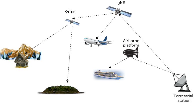


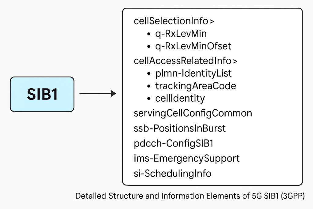


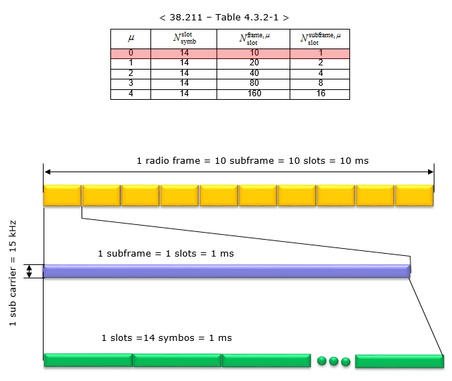
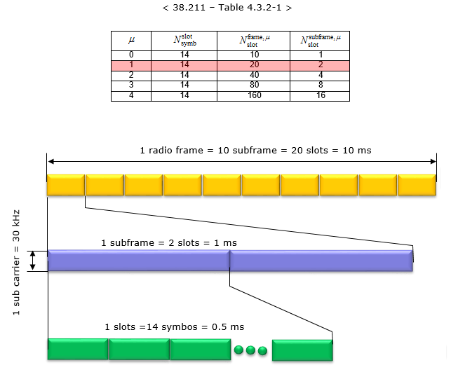
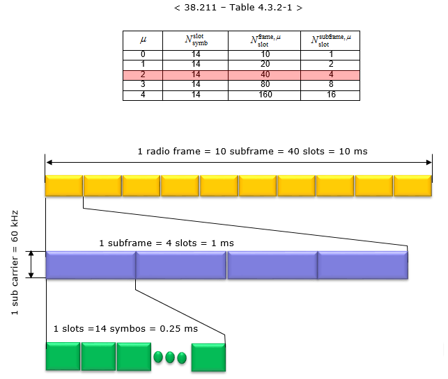
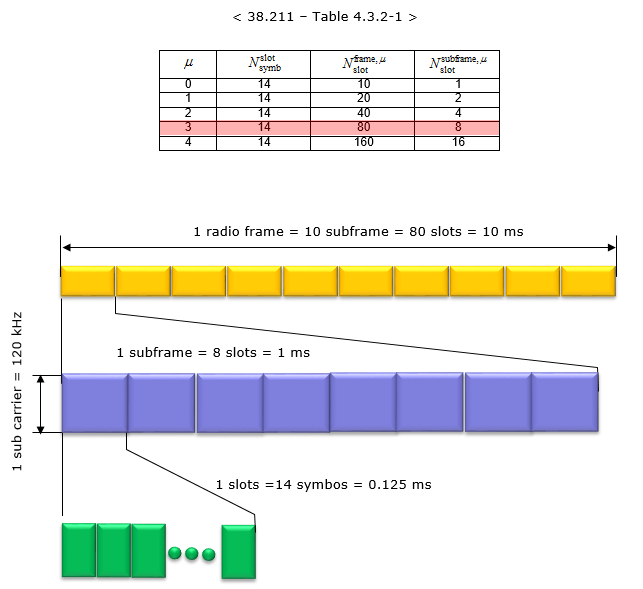
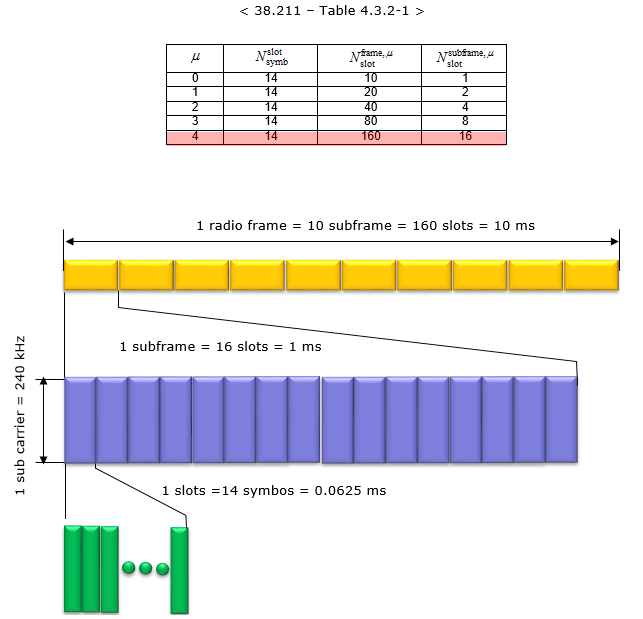
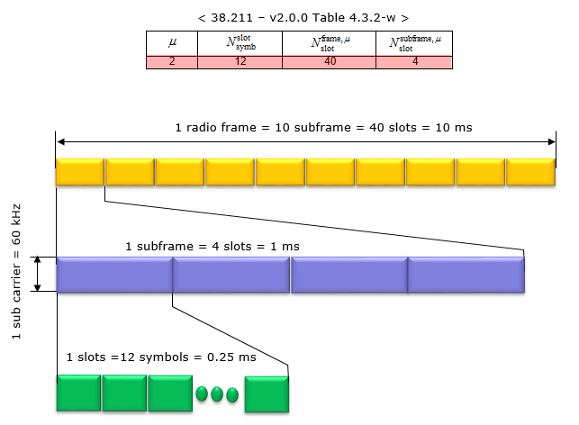

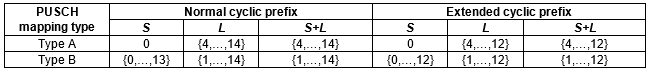


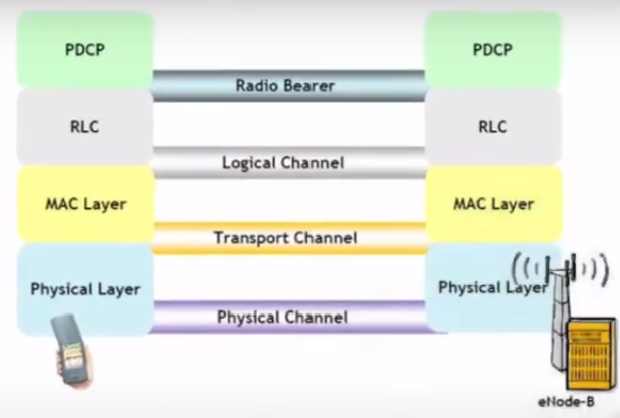


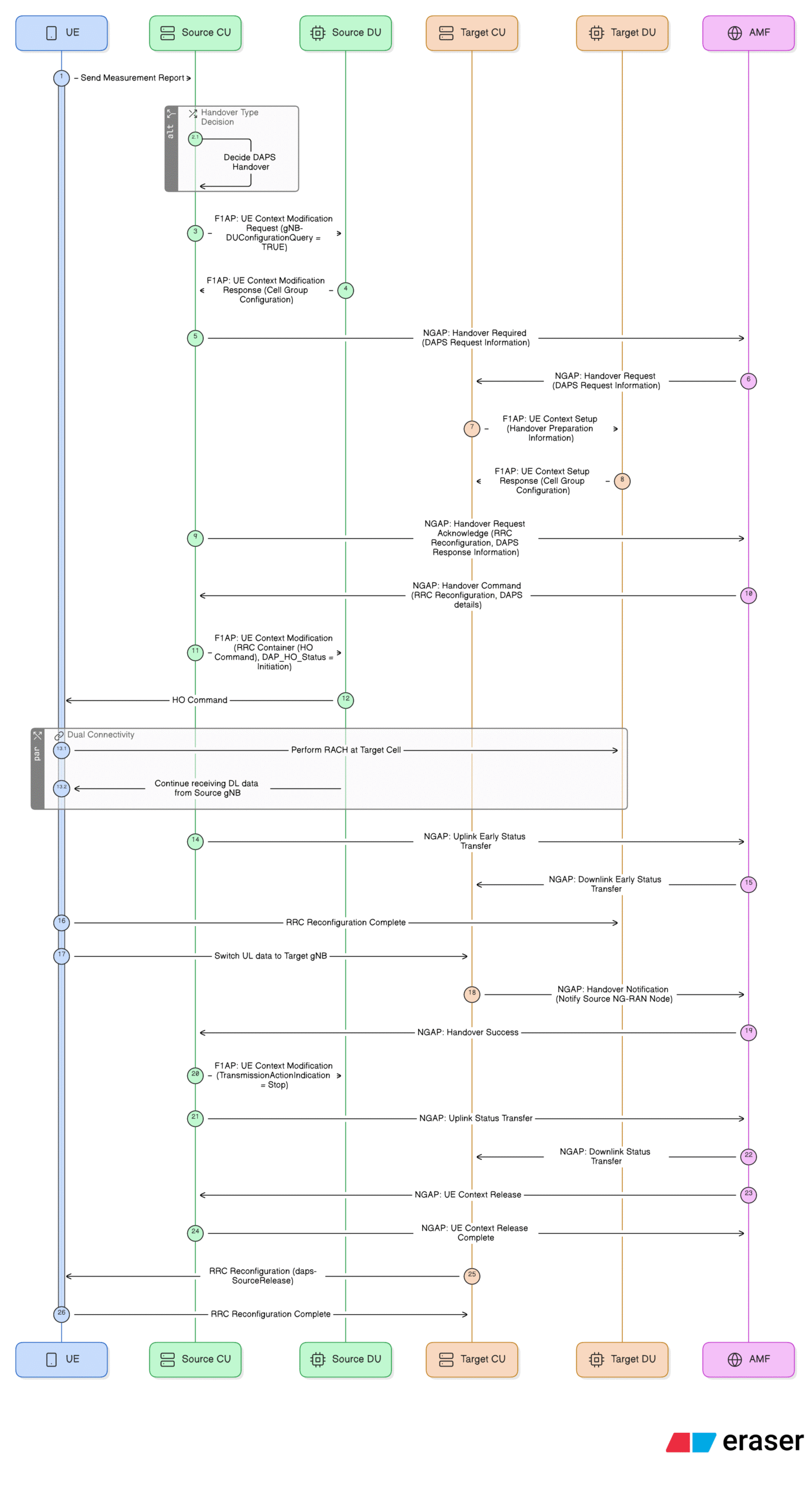
Nice utility. Helpful when away from laptop